Стандартная ошибка предсказания это

Имея
прямую регрессии, необходимо оценить
насколько сильно точки исходных данных
отклоняются от прямой регрессии. Можно
выполнить оценку разброса, аналогичную
стандартному отклонению выборки. Этот
показатель, называемый стандартной
ошибкой оценки, демонстрирует величину
отклонения точек исходных данных от
прямой регрессии в направлении оси Y.
Стандартная ошибка оценки ()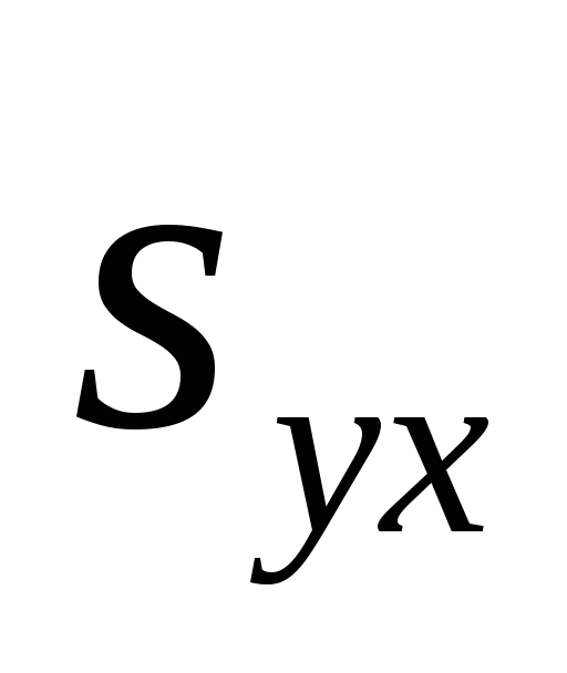
вычисляется по следующей формуле.

Стандартная
ошибка оценки измеряет степень отличия
реальных значений Y от оцененной величины.
Для сравнительно больших выборок следует
ожидать, что около 67% разностей по модулю
не будет превышать

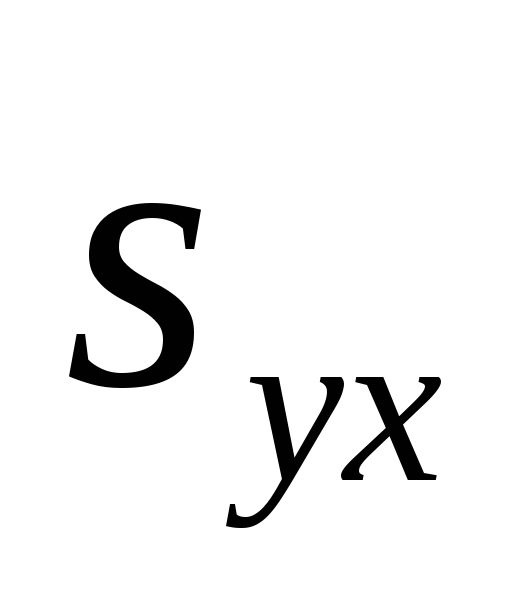
и около 95% модулей разностей будет не
больше 2.

Стандартная
ошибка оценки подобна стандартному
отклонению. Ее можно использовать для
оценки стандартного отклонения
совокупности. Фактически

оценивает стандартное отклонение

слагаемого ошибки

в статистической модели простой линейной
регрессии. Другими словами,

оценивает общее стандартное отклонение

нормального распределения значений Y,
имеющих математические ожидания

для каждого X.

Малая
стандартная ошибка оценки, полученная
при регрессионном анализе, свидетельствует,
что все точки данных находятся очень
близко к прямой регрессии. Если стандартная
ошибка оценки велика, точки данных могут
значительно удаляться от прямой.

2.3 Прогнозирование величины y

Регрессионную
прямую можно использовать для оценки
величины переменной Y
при данных значениях переменной X. Чтобы
получить точечный прогноз, или предсказание
для данного значения X, просто вычисляется
значение найденной функции регрессии
в точке X.

Конечно
реальные значения величины Y,
соответствующие рассматриваемым
значениям величины X, к сожалению, не
лежат в точности на регрессионной
прямой. Фактически они разбросаны
относительно прямой в соответствии с
величиной
.
Более того, выборочная регрессионная
прямая является оценкой регрессионной
прямой генеральной совокупности,
основанной на выборке из определенных
пар данных. Другая случайная выборка
даст иную выборочную прямую регрессии;
это аналогично ситуации, когда различные
выборки из одной и той же генеральной
совокупности дают различные значения
выборочного среднего.

Есть
два источника неопределенности в
точечном прогнозе, использующем уравнение
регрессии.

Неопределенность,
обусловленная отклонением точек данных
от выборочной прямой регрессии.
Неопределенность,
обусловленная отклонением выборочной
прямой регрессии от регрессионной
прямой генеральной совокупности.

Интервальный
прогноз значений переменной Y
можно построить так, что при этом будут
учтены оба источника неопределенности.

Стандартная
ошибка прогноза

дает меру вариативности предсказанного
значения Y
около истинной величины Y
для данного значения X.
Стандартная ошибка прогноза равна:

Стандартная
ошибка прогноза зависит от значения X,
для которого прогнозируется величина
Y.

минимально, когда
,
поскольку тогда числитель в третьем
слагаемом под корнем в уравнении будет
0. При прочих неизменных величинах
большему отличию соответствует большее
значение стандартной ошибки прогноза.

Если
статистическая модель простой линейной
регрессии соответствует действительности,
границы интервала прогноза величины Y
равны:

где

— квантиль распределения Стьюдента с
n-2 степенями свободы ().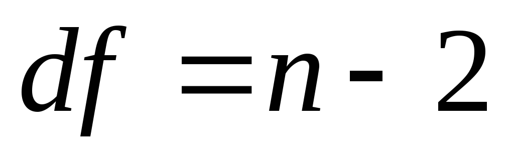
Если выборка велика (),
этот квантиль можно заменить соответствующим
квантилем нормального распределения.
Например, для большой выборки 95%-ный
интервал прогноза задается следующими
значениями:

Завершим
раздел обзором предположений, положенных
в основу статистической модели линейной
регрессии.

Для
заданного значения X генеральная
совокупность значений Y имеет нормальное
распределение относительно регрессионной
прямой совокупности. На практике
приемлемые результаты получаются
и
тогда, когда значения Y имеют
нормальное распределение лишь
приблизительно.
Разброс
генеральной совокупности точек данных
относительно регрессионной прямой
совокупности остается постоянным всюду
вдоль этой прямой. Иными словами, при
возрастании значений X в точках данных
дисперсия генеральной совокупности
не увеличивается и не уменьшается.
Нарушение этого предположения называется
гетероскедастичностью.
Слагаемые
ошибок

независимы между собой. Это предположение
определяет случайность выборки точек
Х-Y.
Если точки данных X-Y
записывались в течение некоторого
времени, данное предположение часто
нарушается. Вместо независимых данных,
такие последовательные наблюдения
будут давать серийно коррелированные
значения.
В
генеральной совокупности существует
линейная зависимость между X и Y.
По аналогии с простой линейной регрессией
может рассматриваться и нелинейная
зависимость между X и У. Некоторые такие
случаи будут обсуждаться ниже.

Соседние файлы в предмете [НЕСОРТИРОВАННОЕ]

Источник

Что такое стандартная ошибка оценки? (Определение и пример)

17 авг. 2022 г.
читать 3 мин

Стандартная ошибка оценки — это способ измерения точности прогнозов, сделанных регрессионной моделью.

Часто обозначаемый σ est , он рассчитывается как:

σ est = √ Σ(y – ŷ) 2 /n

куда:

y: наблюдаемое значение
ŷ: Прогнозируемое значение
n: общее количество наблюдений

Стандартная ошибка оценки дает нам представление о том, насколько хорошо регрессионная модель соответствует набору данных. Особенно:

Чем меньше значение, тем лучше соответствие.
Чем больше значение, тем хуже соответствие.

Для регрессионной модели с небольшой стандартной ошибкой оценки точки данных будут плотно сгруппированы вокруг предполагаемой линии регрессии:

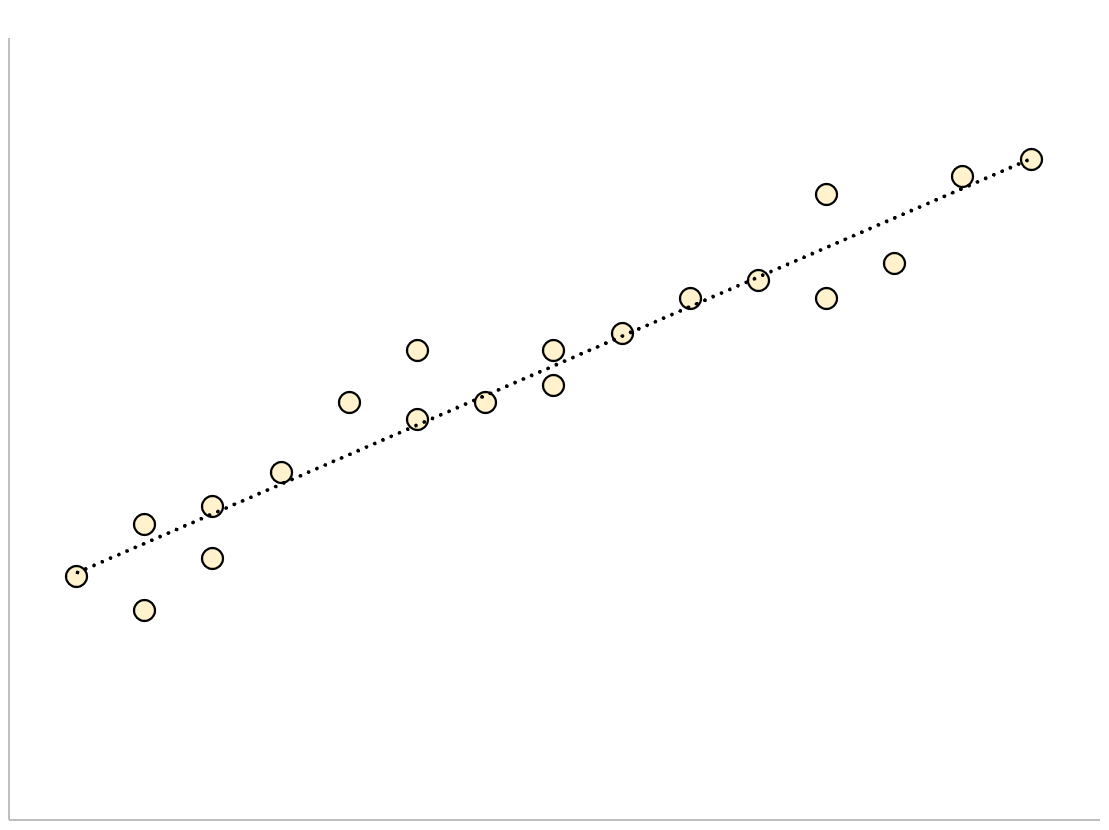
И наоборот, для регрессионной модели с большой стандартной ошибкой оценки точки данных будут более свободно разбросаны по линии регрессии:

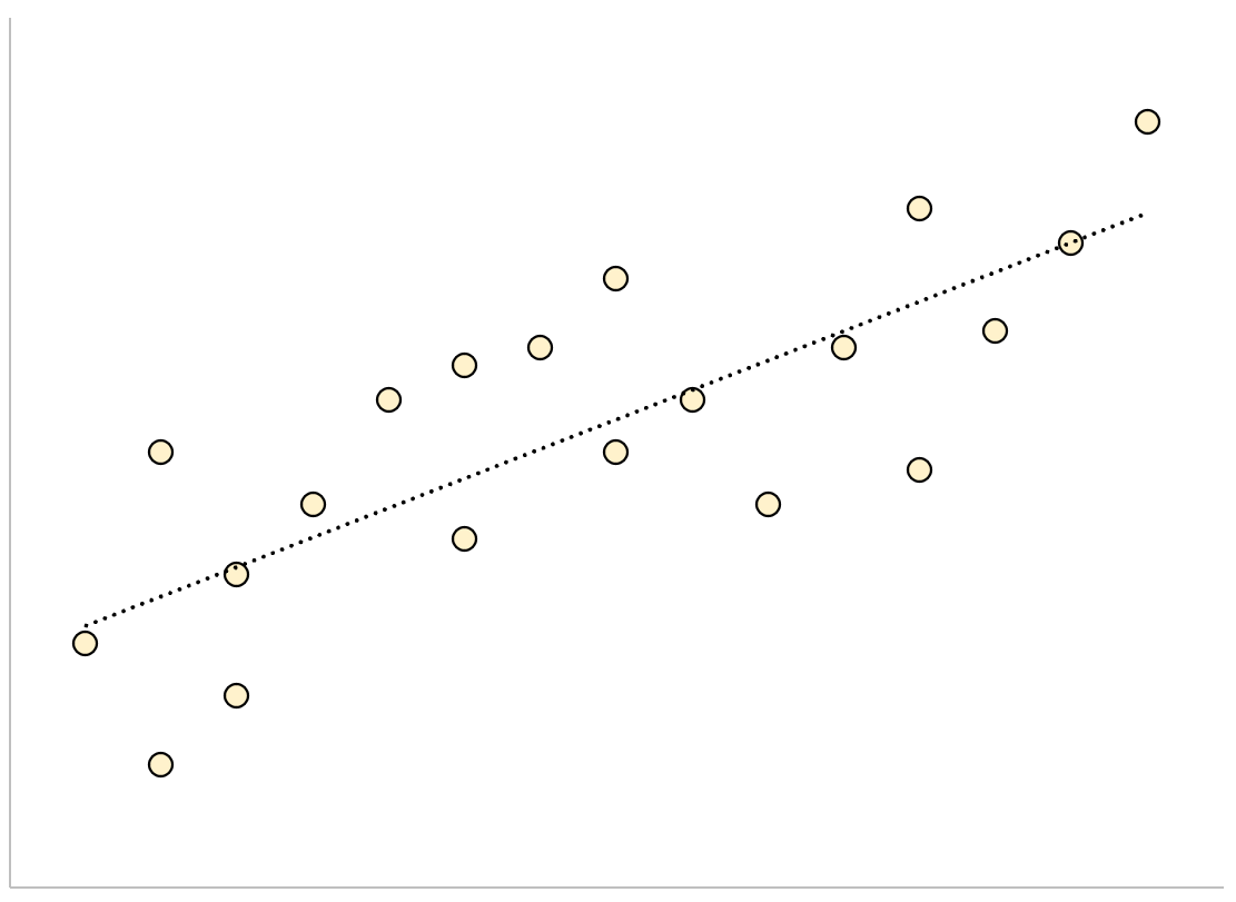
В следующем примере показано, как рассчитать и интерпретировать стандартную ошибку оценки для регрессионной модели в Excel.

Пример: стандартная ошибка оценки в Excel

Используйте следующие шаги, чтобы вычислить стандартную ошибку оценки для регрессионной модели в Excel.

Шаг 1: введите данные

Сначала введите значения для набора данных:

Шаг 2: выполните линейную регрессию

Затем щелкните вкладку « Данные » на верхней ленте. Затем выберите параметр « Анализ данных» в группе « Анализ ».

Если вы не видите эту опцию, вам нужно сначала загрузить пакет инструментов анализа .

В появившемся новом окне нажмите « Регрессия », а затем нажмите « ОК ».

В появившемся новом окне заполните следующую информацию:

Как только вы нажмете OK , появится вывод регрессии:

Мы можем использовать коэффициенты из таблицы регрессии для построения оценочного уравнения регрессии:

ŷ = 13,367 + 1,693 (х)

И мы видим, что стандартная ошибка оценки для этой регрессионной модели оказывается равной 6,006.Проще говоря, это говорит нам о том, что средняя точка данных отклоняется от линии регрессии на 6,006 единицы.

Мы можем использовать оценочное уравнение регрессии и стандартную ошибку оценки, чтобы построить 95% доверительный интервал для прогнозируемого значения определенной точки данных.

Например, предположим, что x равно 10. Используя оценочное уравнение регрессии, мы можем предсказать, что y будет равно:

ŷ = 13,367 + 1,693 * (10) = 30,297

И мы можем получить 95% доверительный интервал для этой оценки, используя следующую формулу:

95% ДИ = [ŷ – 1,96*σ расч ., ŷ + 1,96*σ расч .]

Для нашего примера доверительный интервал 95% будет рассчитываться как:

95% ДИ = [ŷ – 1,96*σ расч ., ŷ + 1,96*σ расч .]
95% ДИ = [30,297 – 1,96*6,006, 30,297 + 1,96*6,006]
95% ДИ = [18,525, 42,069]

Дополнительные ресурсы

Как выполнить простую линейную регрессию в Excel
Как выполнить множественную линейную регрессию в Excel
Как создать остаточный график в Excel

Источник

Ошибка прогнозирования: виды, формулы, примеры

Ошибка прогнозирования — это такая величина, которая показывает, как сильно прогнозное значение отклонилось от фактического. Она используется для расчета точности прогнозирования, что в свою очередь помогает нам оценивать как точно и корректно мы сформировали прогноз. В данной статье я расскажу про основные процентные «ошибки прогнозирования» с кратким описанием и формулой для расчета. А в конце статьи я приведу общий пример расчётов в Excel. Напомню, что в своих расчетах я в основном использую ошибку WAPE или MAD-Mean Ratio, о которой подробно я рассказал в статье про точность прогнозирования, здесь она также будет упомянута.

В каждой формуле буквой Ф обозначено фактическое значение, а буквой П — прогнозное. Каждая ошибка прогнозирования (кроме последней!), может использоваться для нахождения общей точности прогнозирования некоторого списка позиций, по типу того, что изображен ниже (либо для любого другого подобной детализации):

Алгоритм для нахождения любой из ошибок прогнозирования для такого списка примерно одинаковый: сначала находим ошибку прогнозирования по одной позиции, а затем рассчитываем общую. Итак, основные ошибки прогнозирования!

MPE — Mean Percent Error

MPE — средняя процентная ошибка прогнозирования. Основная проблема данной ошибки заключается в том, что в нестабильном числовом ряду с большими выбросами любое незначительное колебание факта или прогноза может значительно поменять показатель ошибки и, как следствие, точности прогнозирования. Помимо этого, ошибка является несимметричной: одинаковые отклонения в плюс и в минус по-разному влияют на показатель ошибки.

Ошибка прогнозирования MPE

Для каждой позиции рассчитывается ошибка прогноза (из факта вычитается прогноз) — Error
Для каждой позиции рассчитывается процентная ошибка прогноза (ошибка прогноза делится на фактический показатель) — Percent Error
Находится среднее арифметическое всех процентных ошибок прогноза (процентные ошибки суммируются и делятся на количество) — Mean Percent Error

MAPE — Mean Absolute Percent Error

MAPE — средняя абсолютная процентная ошибка прогнозирования. Основная проблема данной ошибки такая же, как и у MPE — нестабильность.

Ошибка прогнозирования MAPE

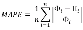
Для каждой позиции рассчитывается абсолютная ошибка прогноза (прогноз вычитается из факта по модулю) — Absolute Error
Для каждой позиции рассчитывается абсолютная процентная ошибка прогноза (абсолютная ошибка прогноза делится на фактический показатель) — Absolute Percent Error
Находится среднее арифметическое всех абсолютных процентных ошибок прогноза (абсолютные процентные ошибки суммируются и делятся на количество) — Mean Absolute Percent Error

Вместо среднего арифметического всех абсолютных процентных ошибок прогноза можно использовать медиану числового ряда (MdAPE — Median Absolute Percent Error), она наиболее устойчива к выбросам.

WMAPE / MAD-Mean Ratio / WAPE — Weighted Absolute Percent Error

WAPE — взвешенная абсолютная процентная ошибка прогнозирования. Одна из «лучших ошибок» для расчета точности прогнозирования. Часто называется как MAD-Mean Ratio, то есть отношение MAD (Mean Absolute Deviation — среднее абсолютное отклонение/ошибка) к Mean (среднее арифметическое). После упрощения дроби получается искомая формула WAPE, которая очень проста в понимании:

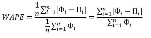
Ошибка прогнозирования WAPE MAD-Mean Ratio

Для каждой позиции рассчитывается абсолютная ошибка прогноза (прогноз вычитается из факта, по модулю) — Absolute Error
Находится сумма всех фактов по всем позициям (общий фактический объем)
Сумма всех абсолютных ошибок делится на сумму всех фактов — WAPE

Данная ошибка прогнозирования является симметричной и наименее чувствительна к искажениям числового ряда.

Рекомендуется к использованию при расчете точности прогнозирования. Более подробно читать здесь.

RMSE (as %) / nRMSE — Root Mean Square Error

RMSE — среднеквадратичная ошибка прогнозирования. Примерно такая же проблема, как и в MPE и MAPE: так как каждое отклонение возводится в квадрат, любое небольшое отклонение может значительно повлиять на показатель ошибки. Стоит отметить, что существует также ошибка MSE, из которой RMSE как раз и получается путем извлечения корня. Но так как MSE дает расчетные единицы измерения в квадрате, то использовать данную ошибку будет немного неправильно.

Ошибка прогнозирования RMSE

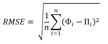
Для каждой позиции рассчитывается квадрат отклонений (разница между фактом и прогнозом, возведенная в квадрат) — Square Error
Затем рассчитывается среднее арифметическое (сумма квадратов отклонений, деленное на количество) — MSE — Mean Square Error
Извлекаем корень из полученного результат — RMSE
Для перевода в процентную или в «нормализованную» среднеквадратичную ошибку необходимо:
1. Разделить на разницу между максимальным и минимальным значением показателей
2. Разделить на разницу между третьим и первым квартилем значений показателей
3. Разделить на среднее арифметическое значений показателей (наиболее часто встречающийся вариант)

MASE — Mean Absolute Scaled Error

MASE — средняя абсолютная масштабированная ошибка прогнозирования. Согласно Википедии, является очень хорошим вариантом для расчета точности, так как сама ошибка не зависит от масштабов данных и является симметричной: то есть положительные и отрицательные отклонения от факта рассматриваются в равной степени.

Важно! Если предыдущие ошибки прогнозирования мы могли использовать для нахождения точности прогнозирования некого списка номенклатур, где каждой из которых соответствует фактическое и прогнозное значение (как было в примере в начале статьи), то данная ошибка для этого не предназначена: MASE используется для расчета точности прогнозирования одной единственной позиции, основываясь на предыдущих показателях факта и прогноза, и чем больше этих показателей, тем более точно мы сможем рассчитать показатель точности. Вероятно, из-за этого ошибка не получила широкого распространения.

Здесь данная формула представлена исключительно для ознакомления и не рекомендуется к использованию.

Суть формулы заключается в нахождении среднего арифметического всех масштабированных ошибок, что при упрощении даст нам следующую конечную формулу:

Ошибка прогнозирования MASE

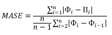
Также, хочу отметить, что существует ошибка RMMSE (Root Mean Square Scaled Error — Среднеквадратичная масштабированная ошибка), которая примерно похожа на MASE, с теми же преимуществами и недостатками.

Это основные ошибки прогнозирования, которые могут использоваться для расчета точности прогнозирования. Но не все! Их очень много и, возможно, чуть позже я добавлю еще немного информации о некоторых из них. А примеры расчетов уже описанных ошибок прогнозирования будут выложены через некоторое время, пока что я подготавливаю пример, ожидайте.

Об авторе

HeinzBr

Автор статей и создатель сайта SHTEM.RU

Источник

Correlation and Regression

Andrew F. Siegel, Michael R. Wagner, in Practical Business Statistics (Eighth Edition), 2022

The Standard Error of Estimate: How Large Are the Prediction Errors?

The standard error of estimate, denoted S_e here (but often denoted S in computer printouts), tells you approximately how large the prediction errors (residuals) are for your data set in the same units as Y. How well can you predict Y? The answer is to within about S_e above or below.¹⁶ Because you usually want your forecasts and predictions to be as accurate as possible, you would be glad to find a small value for S_e. You can interpret S_e as a standard deviation in the sense that if you have a normal distribution for the prediction errors, then you will expect about two-thirds of the data points to fall within a distance S_e either above or below the regression line. Also, about 95% of the data values should fall within 2S_e, and so forth. This is illustrated in Fig. 11.2.10 for the production cost example.

Fig. 11.2.10. The standard error of estimate, S_e, indicates approximately how much error you make when you use the predicted value for Y (on the least-squares line) instead of the actual value of Y. You may expect about two-thirds of the data points to be within S_e above or below the least-squares line for a data set with a normal linear relationship, such as this one.

The standard error of estimate may be found using the following formulas:

Standard Error of Estimate

Se=SY(1−r2)n−1n−2(forcomputation)=1n−2∑i=1n[Yi−(a+bXi)]2(forinterpretation)

The first formula shows how S_e is computed by reducing S_Y according to the correlation and sample size. Indeed, S_e will usually be smaller than S_Y because the line a + bX summarizes the relationship and therefore comes closer to the Y values than does the simpler summary, Y¯. The second formula shows how S_e can be interpreted as the estimated standard deviation of the residuals: The squared prediction errors are averaged by dividing by n − 2 (the appropriate number of degrees of freedom when two numbers, a and b, have been estimated), and the square root undoes the earlier squaring, giving you an answer in the same measurement units as Y.

For the production cost data, the correlation was found to be r = 0.869193, the variability in the individual cost numbers is S_Y = $389.6131, and the sample size is n = 18. The standard error of estimate is therefore

Se=SY(1−r2)n−1n−2=389.6131(1−0.8691932)18−118−2=389.6131(0.0244503)1716=389.61310.259785=$198.58

This tells you that, for a typical week, the actual cost was different from the predicted cost (on the least-squares line) by about $198.58. Although the least-squares prediction line takes full advantage of the relationship between cost and number produced, the predictions are far from perfect.

Read full chapter

URL:

https://www.sciencedirect.com/science/article/pii/B9780128200254000117

Detection of a Trend in Population Estimates

William L. Thompson, … Charles Gowan, in Monitoring Vertebrate Populations, 1998

5.2 VARIANCE COMPONENTS

In this section, we discuss sources of variation that must be considered to make inferences from data when trying to detect trends. Three sources of variation must be considered: sampling variation, temporal variation in the population dynamics process, and spatial variation in the dynamics of the population across space. The latter two sources often are referred to as process variation, i.e., variation in the population dynamics process associated with environmental variation (such as rainfall, temperature, community succession, fires, or elevation). Methods to separate process variation from sampling variation will be presented.

Detection of a trend in a population’s size requires at least two abundance estimates. For example, if the population size of Mexican spotted owls in Mesa Verde National Park is determined as 50 pairs in 1990, and as only 10 pairs in 1995, we would be concerned that a significant negative trend in the population exists during this time period, and that action must be taken to alleviate the trend. However, if the 1995 estimate was 40 pairs, we might still be concerned, but would be less confident that immediate action is required. Two sources of variation must be assessed before we are confident of our inference from these estimates.

The first source of variation is the uncertainty we have in our population estimates. We want to be sure that the two estimates are different, i.e., the difference between the two estimates is greater than would be expected from chance alone because of the sampling errors associated with each estimate. Typically, we present our uncertainty in our estimate as its variance, and use this variance to generate a confidence interval for our estimate. Suppose that the 1990 estimate of Nˆ90 = 50 pairs has a sampling variance of Vaˆr(Nˆ90)=25. Then, under the assumption of the estimate being normally distributed with a large sample size (i.e., large degrees of freedom), we would compute a 95% confidence interval as 50 ± 1.96 25, or 40.2–59.8. If the 1995 estimate was Nˆ95 = 40 with a sampling variance of Vâr(Nˆ95) = 20, then the 95% confidence interval for this estimate is 40 ± 1.96 20, or 31.2–48.8. Based on the overlap of the two confidence intervals (Fig. 5.2), we would conclude that by chance alone, these two estimates are probably not different. We also could compute a simple test as

Figure 5.2. The 95% confidence intervals plotted with the 1990 and 1995 population estimates.

(5.3)z=Nˆ90−Nˆ95Vaˆr(Nˆ90)+Vaˆr(Nˆ95),

which for this example results in z = 1.491, with a probability of observing a z statistic this large or larger of P = 0.136. Although we might be alarmed, the chances are that 13.6 times out of 100 we would observe this large of a change just by random chance.

A variation of the previous test is commonly conducted for several reasons: (1) we often are interested in the ratio of two population estimates (rather than the difference) because a ratio represents the rate of change of the population, (2) the variance of Nˆ is usually linked to its estimate by Vaˆr(Nˆ)=NˆC (e.g., Skalski and Robson, 1992, pp. 28–29), and (3) ln(Nˆ) is more likely to be normally distributed than Nˆ. Fortuitously, a log transformation provides some correction to all three of the above reasons and results in a more efficient statistical procedure. Because

(5.4)Var[ln(Nˆ)]=Var(Nˆ)Nˆ2,

we construct the z test as

(5.5)z=ln(Nˆ90)−ln(Nˆ95)Vaˆr[ln(Nˆ90)]+Vaˆr[ln(Nˆ95)]

to provide a more efficient (i.e., more powerful) test.

Suppose we had made a much more intensive effort in sampling the owl population, so that the sampling variances were one-half of the values observed (which would generally take about 4 times the effort). Thus, Vâr(Nˆ90) = 12.5 and Vâr(Nˆ95) = 10, giving a z statistic of 2.108 with probability value of P = 0.035. Now, we would conclude that the owl population was lower in 1995 than in 1990, and that this difference is unlikely due to variation in our samples, i.e., that an actual reduction in population size has taken place.

This leads us to the second variance component associated with determining whether a trend in the population is important. We would expect the size of the owl population (and any other population, for that matter) to fluctuate through time. How can we determine if this reduction is important? The answer lies in determining what the variation in the owl population has been for some period of time in the past, and then if the observed reduction is outside the range expected from this past fluctuation. Consider the example in Fig. 5.3, where the true population size (no sampling variation) is plotted. The population fluctuates around a mean of 50, but values more extreme than the range 40 to 60 are common. Note that a decline from 76 to 29 pairs occurred from 1984 to 1985, and that declines from over 50 pairs to under 40 pairs are fairly common occurrences. Thus, based on our previous example, a decline from 50 to 40 is not at all unreasonable given the past population dynamics of this hypothetical population.

Figure 5.3. Actual number of pairs of owls that exist each year. In reality, we never know these values, and can only estimate them.

To determine the level of change in population size that should receive our attention and suggest management action, we need to know something about the temporal variation in the population. The only way to estimate this variance component is to observe the population across a number of years. The exact number of years will depend on the magnitude of the temporal variation. Thus, if the population does not change much from year to year, a few observations will show this consistency. On the other hand, if the population fluctuates a lot, as in Fig. 5.3, many years of observations are needed to estimate the temporal variance. For the example in Fig. 5.3, we could compute the temporal variance as the variance of the 15 years. We find a variance of 265.7, or a standard deviation of 16.3 (Example 5.1). With a SD of 16.3, we would expect roughly 95% of the population values to be in the range of ±2 SD of the mean population size. This inference is based on the population being stable, i.e., not having an upward or downward trend, and being roughly normally distributed. For a normal distribution, 95% of the values lie in the interval ±2 SD of the mean. Therefore, a change of 2 SD, or 32.6, is not a particularly big change given the temporal variation observed over the 15-year period. Such a change should occur with probability greater than 1/20, or 0.05.

A complicating problem with estimating the temporal variance of a population’s size is that we are seldom allowed to observe the true value of the population size. Rather, we are required to sample the population, and hence only obtain an estimate of the population size each year, with its associated sampling variance. Thus, we would need to include the 95% confidence bars on the annual estimates. As a result of this uncertainty from our sampling procedure, we would conclude that many of the year-to-year changes were not really changes because the estimates were not different. This complication leads to a further problem. If we compute the variance with the usual formula when estimates of population size replace the actual population size shown in Fig. 5.3, we obtain a variance estimate larger than the true temporal variance because our sampling uncertainty is included in the variance. For low levels of sampling effort each year, we would have a high sampling variance associated with each estimate, and as a result, we would have a high variance across years. The noise associated with our low sampling intensity would suggest that the population is fluctuating widely, when in fact the population could be constant (i.e., temporal variance is zero), and the estimated changes in the population are just due to sampling variance.

This mixture of sampling and temporal variation becomes particularly important in population viability analysis (PVA). The objective of a PVA is to estimate the probability of extinction for a population, given current size, and some idea of the variation in the population dynamics (i.e., temporal variation). If our estimate of temporal variation includes sampling variation, and the level of effort to obtain the estimates is relatively low, the high sampling variation causes our naive estimate of temporal variation to be much too large. When we apply our PVA analysis with this inflated estimate of temporal variance, we conclude that the population is much more likely to go extinct than it really is, and hence the importance of separating sampling variation from process variation.

Typically, we estimate variance components with analysis of variance (ANOVA) procedures. For the example considered here, we would have to have at least two estimates of population size for a series of years to obtain valid estimates of sampling and temporal variation. Further, typical ANOVA techniques assume that the sampling variation is constant, and so do not account for differences in levels of effort, or the fact that sampling variance is usually a function of population size. For our example, we have an estimate of sampling variance for each of our estimates, obtained from the population estimation methods considered in this manual. That is, capture–recapture, mark–resight, line transects, removal methods, and quadrat counts all produce estimates of sampling variation. Thus, we do not want to estimate sampling variation by obtaining replicate estimates, but want to use the available estimate. Therefore, we present a method of moments estimator developed in Burnham et al. (1987, Part 5). Skalski and Robson (1992, Chapter 2) also present a similar procedure, but do not develop the weighted estimator presented here.

Example 5.1 Population Size, Estimates, Standard Error of the Estimates, and Confidence Intervals for Owl Pairs in Fig. 5.3

			Standard
Year	Population	Estimate	error	Lower 95% CI	Upper 95% CI
1980	44	40.04	5.926	28.42	51.66
1981	48	50.51	11.004	28.94	72.08
1982	61	61.36	15.278	31.42	91.31
1983	48	47.6	11.062	25.92	69.28
1984	76	95.51	18.988	58.3	132.72
1985	29	33.81	8.803	16.56	51.06
1986	60	34.39	5.804	23.01	45.76
1987	59	38.52	11.168	16.63	60.41
1988	76	84.57	21.312	42.8	126.34
1989	42	30.04	6.918	16.48	43.6
1990	29	20.29	7.529	5.54	35.05
1991	68	68.42	17.969	33.2	103.64
1992	42	45.51	13.225	19.6	71.44
1993	27	27.01	6.137	14.98	39.04
1994	72	71.12	14.511	42.67	99.56
1995	54	51.45	8.054	35.66	67.24

The variance of the n = 16 populations is 265.628, whereas the variance of the 16 estimates is 450.376. Sampling variation causes the estimates to have a larger variance than the actual population. The difference of these two variances is an estimate of the sampling variation, i.e., 450.376 – 265.628 = 184.748. The square root of 184.748 is 13.592, and is the approximate mean of the 16 reported standard errors.

To obtain an unbiased estimate of the temporal variance, we must remove the sampling variation from the estimate of the total variance. Define σtotal2 as the total variance, estimated for n = 16 estimates of owl pairs (Nˆi, i = 1980, …, 1995) as

(5.6)σˆtotal2=Σi=19801995(Nˆi−N¯)2(n−1)=Σi=19801995Nˆi2(Σi−19801985Nˆi)2n(n−1),

where the symbol indicates the estimate of the parameter. Thus, Nˆi are the estimates of the actual populations, N_i, and σˆtotal2 is an estimate of the total variance σˆi2 For each estimate, Nˆi, we also have an associated sampling variance, σˆi2. Then, a simple estimator of the temporal variance, σ²_time, is given by

(5.7)σˆtime2=σˆtotal2−Σi=19801995σˆi2n,

when we can assume that all of the sampling variances, σˆi2, are equal. The above equation corresponds to Eq. (2.6) of Skalski and Robson (1992). When the σˆi2 cannot all be assumed to be equal, a more complex calculation is required (Burnham et al., 1987, Section 4.3) because each estimate must be weighted by its sampling variance. We take as the weight of each estimate the reciprocal of the sum of temporal variance plus the sampling variance, 1/(σˆtime2+σˆi2). That is, Var(Nˆi)=σˆtime2+σˆi2, so wi=1/Var(Nˆi)=1/(σˆtime2+σˆi2). Then, the weighted total variance is computed as

(5.8)σˆtotal2=Σi=19801995wi(Nˆi−N¯)2(n−1)Σi=19801995wi

with the mean of the estimates now computed as a weighted mean,

(5.9)N¯=Σi=19801995wiNˆiΣi=19801995wi.

We now know that the theoretical variance N¯ is

(5.10)Var(N¯)=Var(Σi=19801995wiNˆiΣi=19801995wi)=1Σi=19801995wi

and the empirical variance estimator is Eq. (5.8). Setting these two equations equal,

(5.11)1Σi=19801995wi=Σi=19801995wi(Nˆi−N¯)2(n−1)Σi=19801995wi

(5.12)1=Σi=19801995wi(Nˆi−N¯)2(n−1).

Because we cannot solve for σˆtime2 directly, we have to use an iterative numerical approach to estimate σˆtime2 This procedure involves substituting values of σˆtime2 into Eq. (5.12) via the w_i until the two sides are equal. When both sides are the same, we have our estimate of σˆtime2. Using this estimate of σˆtime2, we can now decide what level of change in Nˆi to Nˆi+1 is important and deserves attention. If the change from a series of estimates is greater than 2σˆtime2, we may want to take action.

Typically, we do not have the luxury of enough background data to estimate σˆtime2, so we end up trying to evaluate whether a series of estimated population sizes is in fact signaling a decline in the population when both sampling and process variance are present. Note that just because we see a decline of the estimates for 3–4 consecutive years, we cannot be sure that the population is actually in a serious decline without knowledge of the mean population size and the temporal variation prior to the decline. Usually, however, we do not have good knowledge of the population size prior to some observed decline, and make a decision to act based on biological perceptions. Keep in mind the kinds of trends displayed in Fig. 5.1. Is the suggested trend part of a cycle, or are we observing a real change in population size? In this discussion, we have only considered temporal variation. A similar procedure can be used to separate spatial variation from sampling variation.

Read full chapter

URL:

https://www.sciencedirect.com/science/article/pii/B9780126889604500058

Multiple Regression

Andrew F. Siegel, Michael R. Wagner, in Practical Business Statistics (Eighth Edition), 2022

Typical Prediction Error: Standard Error of Estimate

Just as for simple regression, with only one X, the standard error of estimate indicates the approximate size of the prediction errors. For the magazine ads example, S_e = $106,072. This tells you that actual page costs for these magazines are typically within about $106,072 from the predicted page costs, in the sense of a standard deviation. That is, if the error distribution is normal, then you would expect about two-thirds of the actual page costs to be within S_e of the predicted page costs, about 95% to be within 2S_e, and so forth.

The standard error of estimate, S_e = $106,072, indicates the remaining variation in page costs after you have used the X variables (audience, percent male, and median income) in the regression equation to predict page costs for each magazine. Compare this to the ordinary univariate standard deviation, S_Y = $163,549, for the page costs, computed by ignoring all the other variables. This standard deviation, S_Y, indicates the remaining variation in page costs after you have used only Y¯ to predict the page costs for each magazine. Note that S_e = $106,072 is smaller than S_Y = $163,549; your errors are typically smaller if you use the regression equation instead of just Y¯ to predict page costs. This suggests that the X variables are helpful in explaining page costs.

Think of the situation this way. If you knew nothing of the X variables, you would use the average page costs (Y¯=$187,628) as your best guess, and you would be wrong by about S_Y = $163,549. But if you knew the audience, percent male readership, and median reader income, you could use the regression equation to find a prediction for page costs that would be wrong by only S_e = $106,072. This reduction in prediction error (from $163,549 to $106,072) is one of the helpful payoffs from running a regression analysis.

Read full chapter

URL:

https://www.sciencedirect.com/science/article/pii/B9780128200254000129

Multiple Regression

Gary Smith, in Essential Statistics, Regression, and Econometrics, 2012

Confidence Intervals for the Coefficients

If the error term is normally distributed and satisfies the four assumptions detailed in the simple regression chapter, the estimators are normally distributed with expected values equal to the parameters they estimate:

a∼N[α, standard deviation of a]bi∼N[βi, standard deviation of bi]

To compute the standard errors (the estimated standard deviations) of these estimators, we need to use the standard error of estimate (SEE) to estimate the standard deviation of the error term:

(10.3)SEE=∑(Y−Y^)2n−(k+1)

Because n observations are used to estimate k + 1 parameters, we have n − (k + 1) degrees of freedom. After choosing a confidence level, such as 95 percent, we use the t distribution with n − (k + 1) degrees of freedom to determine the value t* that corresponds to this probability. The confidence interval for each coefficient is equal to the estimate plus or minus the requisite number of standard errors:

(10.4)a±t*(standard error ofa)bi±t*(standard error ofbi)

For our consumption function, statistical software calculates SEE = 59.193 and these standard errors:

standard error ofa=27.327standard error ofb1=0.019standard error ofb2=0.003

With 49 observations and 2 explanatory variables, we have 49 − (2 + 1) = 46 degrees of freedom. Table A.2 gives t* = 2.013 for a 95 percent confidence interval, so that 95 percent confidence intervals are

α:a±t*(standard error ofa)=−110.126±2.013(27.327)=−110.126±55.010β1:b1±t*(standard error ofb1)=0.798±2.013(0.019)=0.798±0.039β2:b2±t*(standard error ofb2)=0.026±2.013(0.003)=0.026±0.006

Read full chapter

URL:

https://www.sciencedirect.com/science/article/pii/B9780123822215000106

Multiple Regression

Gary Smith, in Essential Statistics, Regression, and Econometrics (Second Edition), 2015

Confidence Intervals for the Coefficients

a∼N[α,standarddeviationofa]bi∼N[βistandarddeviationofbi]

To compute the standard errors (the estimated standard deviations) of these estimators, we need to use the standard error of estimate (SEE) to estimate the standard deviation of the error term:

(10.5)SEE=∑(y−yˆ)2n−(k+1)

Because n observations are used to estimate k + 1 parameters, we have n − (k + 1) degrees of freedom. After choosing a confidence level, such as 95 percent, we use the t distribution with n − (k + 1) degrees of freedom to determine the value t^∗ that corresponds to this probability. The confidence interval for each coefficient is equal to the estimate plus or minus the requisite number of standard errors:

(10.6)a±t∗(standarderrorofa)bi±t∗(standarderrorofbi)

For our consumption function, statistical software calculates SEE = 59.193 and these standard errors:

standarderrorofa=27.327standarderrorofb1=0.019standarderrorofb2=0.003

With 49 observations and two explanatory variables, we have 49 − (2 + 1) = 46 degrees of freedom. Table A.2 gives t^∗ = 2.013 for a 95 percent confidence interval, so that 95 percent confidence intervals are:

α:a±t∗(standarderrorofa)=−110.126±2.013(27.327)=−110.126±55.010β1:b1±t∗(standarderrorofb1)=0.798±2.013(0.019)=0.798±0.039β2:b2±t∗(standarderrorofb2)=0.026±2.013(0.003)=0.026±0.006

Read full chapter

URL:

https://www.sciencedirect.com/science/article/pii/B9780128034590000108

Simple Regression

Gary Smith, in Essential Statistics, Regression, and Econometrics (Second Edition), 2015

Abstract

The simple regression model assumes a linear relationship, Y = α + βX + ε, between a dependent variable Y and an explanatory variable X, with the error term ε encompassing omitted factors. The least squares estimates a and b minimize the sum of squared errors when the fitted line is used to predict the observed values of Y. The standard error of estimate (SEE) is our estimate of the standard deviation of the error term. The standard errors of the estimates a and b can be used to construct confidence intervals for α and β and test null hypotheses, most often that the value of β is zero (Y and X are not linearly related). The coefficient of determination R² compares the model’s sum of the squared prediction errors to the sum of the squared deviations of Y about its mean, and can be interpreted as the fraction of the variation in the dependent variable that is explained by the regression model. The correlation coefficient is equal to the square root of R².

Read full chapter

URL:

https://www.sciencedirect.com/science/article/pii/B978012803459000008X

Bootstrap Method

K. Singh, M. Xie, in International Encyclopedia of Education (Third Edition), 2010

Approximating Standard Error of a Sample Estimate

Let us suppose, information is sought about a population parameter θ. Suppose θˆ is a sample estimator of θ based on a random sample of size n, that is, θˆ is a function of the data (X₁, X₂, …,X_n). In order to estimate standard error of θˆ, as the sample varies over the class of all possible samples, one has the following simple bootstrap approach.

Computeθ1*,θ2*,…,θN*, using the same computing formula as the one used for θˆ, but now base it on N different bootstrap samples (each of size n). A crude recommendation for the size N could be N = n² (in our judgment), unless n² is too large. In that case, it could be reduced to an acceptable size, say nlogen. One defines

SEB(θˆ)=[(1/N)∑i=1N(θi*−θˆ)2]1/2

following the philosophy of bootstrap: replace the population by the empirical population.

An older resampling technique used for this purpose is Jackknife, though bootstrap is more widely applicable. The famous example where Jackknife fails while bootstrap is still useful is that of θˆ = the sample median.

Read full chapter

URL:

https://www.sciencedirect.com/science/article/pii/B9780080448947013099

Pearson, Karl

M. Eileen Magnello, in Encyclopedia of Social Measurement, 2005

The Biometric School

Although Pearson’s success in attracting such large audiences in his Gresham lectures may have played a role in encouraging him to further develop his work in biometry, he resigned from the Gresham Lectureship due to his doctor’s recommendation. Following the success of his Gresham lectures, Pearson began to teach statistics to students at UCL in October 1894. Not only did Galton’s work on his law of ancestral heredity enable Pearson to devise the mathematical properties of the product– moment correlation coefficient (which measures the relationship between two continuous variables) and simple regression (used for the linear prediction between two continuous variables) but also Galton’s ideas led to Pearson’s introduction of multiple correlation and part correlation coefficients, multiple regression and the standard error of estimate (for regression), and the coefficient of variation. By then, Galton had determined graphically the idea of correlation and regression for the normal distribution only. Because Galton’s procedure for measuring correlation involved measuring the slope of the regression line (which was a measure of regression instead), Pearson kept Galton’s “r” to symbolize correlation. Pearson later used the letter b (from the equation for a straight line) to symbolize regression. After Weldon had seen a copy of Pearson’s 1896 paper on correlation, he suggested to Pearson that he should extend the range for correlation from 0 to +1 (as used by Galton) so that it would include all values from −1 to +1.

Pearson achieved a mathematical resolution of multiple correlation and multiple regression, adumbrated in Galton’s law of ancestral heredity in 1885, in his seminal paper Regression, Heredity, and Panmixia in 1896, when he introduced matrix algebra into statistical theory. (Arthur Cayley, who taught at Cambridge when Pearson was a student, created matrix algebra by his discovery of the theory of invariants during the mid-19th century.) Pearson’s theory of multiple regression became important to his work on Mendel in 1904 when he advocated a synthesis of Mendelism and biometry. In the same paper, Pearson also introduced the following statistical methods: eta (η) as a measure for a curvilinear relationship, the standard error of estimate, multiple regression, and multiple and part correlation. He also devised the coefficient of variation as a measure of the ratio of a standard deviation to the corresponding mean expressed as a percentage.

By the end of the 19th century, he began to consider the relationship between two discrete variables, and from 1896 to 1911 Pearson devised more than 18 methods of correlation. In 1900, he devised the tetrachoric correlation and the phi coefficient for dichotomous variables. The tetrachoric correlation requires that both X and Y represent continuous, normally distributed, and linearly related variables, whereas the phi coefficient was designed for so-called point distributions, which implies that the two classes have two point values or merely represent some qualitative attribute. Nine years later, he devised the biserial correlation, where one variable is continuous and the other is discontinuous. With his son Egon, he devised the polychoric correlation in 1922 (which is very similar to canonical correlation today). Although not all of Pearson’s correlational methods have survived him, a number of these methods are still the principal tools used by psychometricians for test construction. Following the publication of his first three statistical papers in Philosophical Transactions of the Royal Society, Pearson was elected a fellow of the Royal Society in 1896. He was awarded the Darwin Medal from the Royal Society in 1898.

Read full chapter

URL:

https://www.sciencedirect.com/science/article/pii/B0123693985002280

Источник

Correlation and Regression

Andrew F. Siegel, Michael R. Wagner, in Practical Business Statistics (Eighth Edition), 2022

The Standard Error of Estimate: How Large Are the Prediction Errors?

The standard error of estimate may be found using the following formulas:

Standard Error of Estimate

Se=SY(1−r2)n−1n−2(forcomputation)=1n−2∑i=1n[Yi−(a+bXi)]2(forinterpretation)

Se=SY(1−r2)n−1n−2=389.6131(1−0.8691932)18−118−2=389.6131(0.0244503)1716=389.61310.259785=$198.58

Read full chapter

URL:

https://www.sciencedirect.com/science/article/pii/B9780128200254000117

Detection of a Trend in Population Estimates

William L. Thompson, … Charles Gowan, in Monitoring Vertebrate Populations, 1998

5.2 VARIANCE COMPONENTS

Figure 5.2. The 95% confidence intervals plotted with the 1990 and 1995 population estimates.

(5.3)z=Nˆ90−Nˆ95Vaˆr(Nˆ90)+Vaˆr(Nˆ95),

(5.4)Var[ln(Nˆ)]=Var(Nˆ)Nˆ2,

we construct the z test as

(5.5)z=ln(Nˆ90)−ln(Nˆ95)Vaˆr[ln(Nˆ90)]+Vaˆr[ln(Nˆ95)]

to provide a more efficient (i.e., more powerful) test.

Figure 5.3. Actual number of pairs of owls that exist each year. In reality, we never know these values, and can only estimate them.

Example 5.1 Population Size, Estimates, Standard Error of the Estimates, and Confidence Intervals for Owl Pairs in Fig. 5.3

			Standard
Year	Population	Estimate	error	Lower 95% CI	Upper 95% CI
1980	44	40.04	5.926	28.42	51.66
1981	48	50.51	11.004	28.94	72.08
1982	61	61.36	15.278	31.42	91.31
1983	48	47.6	11.062	25.92	69.28
1984	76	95.51	18.988	58.3	132.72
1985	29	33.81	8.803	16.56	51.06
1986	60	34.39	5.804	23.01	45.76
1987	59	38.52	11.168	16.63	60.41
1988	76	84.57	21.312	42.8	126.34
1989	42	30.04	6.918	16.48	43.6
1990	29	20.29	7.529	5.54	35.05
1991	68	68.42	17.969	33.2	103.64
1992	42	45.51	13.225	19.6	71.44
1993	27	27.01	6.137	14.98	39.04
1994	72	71.12	14.511	42.67	99.56
1995	54	51.45	8.054	35.66	67.24

(5.6)σˆtotal2=Σi=19801995(Nˆi−N¯)2(n−1)=Σi=19801995Nˆi2(Σi−19801985Nˆi)2n(n−1),

(5.7)σˆtime2=σˆtotal2−Σi=19801995σˆi2n,

(5.8)σˆtotal2=Σi=19801995wi(Nˆi−N¯)2(n−1)Σi=19801995wi

with the mean of the estimates now computed as a weighted mean,

(5.9)N¯=Σi=19801995wiNˆiΣi=19801995wi.

We now know that the theoretical variance N¯ is

(5.10)Var(N¯)=Var(Σi=19801995wiNˆiΣi=19801995wi)=1Σi=19801995wi

and the empirical variance estimator is Eq. (5.8). Setting these two equations equal,

(5.11)1Σi=19801995wi=Σi=19801995wi(Nˆi−N¯)2(n−1)Σi=19801995wi

(5.12)1=Σi=19801995wi(Nˆi−N¯)2(n−1).

Read full chapter

URL:

https://www.sciencedirect.com/science/article/pii/B9780126889604500058

Multiple Regression

Andrew F. Siegel, Michael R. Wagner, in Practical Business Statistics (Eighth Edition), 2022

Typical Prediction Error: Standard Error of Estimate

Read full chapter

URL:

https://www.sciencedirect.com/science/article/pii/B9780128200254000129

Multiple Regression

Gary Smith, in Essential Statistics, Regression, and Econometrics, 2012

Confidence Intervals for the Coefficients

a∼N[α, standard deviation of a]bi∼N[βi, standard deviation of bi]

To compute the standard errors (the estimated standard deviations) of these estimators, we need to use the standard error of estimate (SEE) to estimate the standard deviation of the error term:

(10.3)SEE=∑(Y−Y^)2n−(k+1)

(10.4)a±t*(standard error ofa)bi±t*(standard error ofbi)

For our consumption function, statistical software calculates SEE = 59.193 and these standard errors:

standard error ofa=27.327standard error ofb1=0.019standard error ofb2=0.003

Read full chapter

URL:

https://www.sciencedirect.com/science/article/pii/B9780123822215000106

Multiple Regression

Gary Smith, in Essential Statistics, Regression, and Econometrics (Second Edition), 2015

Confidence Intervals for the Coefficients

a∼N[α,standarddeviationofa]bi∼N[βistandarddeviationofbi]

To compute the standard errors (the estimated standard deviations) of these estimators, we need to use the standard error of estimate (SEE) to estimate the standard deviation of the error term:

(10.5)SEE=∑(y−yˆ)2n−(k+1)

Because n observations are used to estimate k + 1 parameters, we have n − (k + 1) degrees of freedom. After choosing a confidence level, such as 95 percent, we use the t distribution with n − (k + 1) degrees of freedom to determine the value t^∗ that corresponds to this probability. The confidence interval for each coefficient is equal to the estimate plus or minus the requisite number of standard errors:

(10.6)a±t∗(standarderrorofa)bi±t∗(standarderrorofbi)

For our consumption function, statistical software calculates SEE = 59.193 and these standard errors:

standarderrorofa=27.327standarderrorofb1=0.019standarderrorofb2=0.003

Read full chapter

URL:

https://www.sciencedirect.com/science/article/pii/B9780128034590000108

Simple Regression

Gary Smith, in Essential Statistics, Regression, and Econometrics (Second Edition), 2015

Abstract

Read full chapter

URL:

https://www.sciencedirect.com/science/article/pii/B978012803459000008X

Bootstrap Method

K. Singh, M. Xie, in International Encyclopedia of Education (Third Edition), 2010

Approximating Standard Error of a Sample Estimate

SEB(θˆ)=[(1/N)∑i=1N(θi*−θˆ)2]1/2

following the philosophy of bootstrap: replace the population by the empirical population.

Read full chapter

URL:

https://www.sciencedirect.com/science/article/pii/B9780080448947013099

Pearson, Karl

M. Eileen Magnello, in Encyclopedia of Social Measurement, 2005

The Biometric School

Read full chapter

URL:

https://www.sciencedirect.com/science/article/pii/B0123693985002280

Источник

В зависимости от контекста термин «прогнозирование» в эконометрике может трактоваться по-разному. Применительно к данным временных рядов речь обычно идет о прогнозировании будущего значения зависимой переменной, например, курса рубля или ВВП. Когда же речь идет о пространственных выборках, под прогнозированием понимают предсказание значения зависимой переменной для заданных значений объясняющих переменных. Например, предсказание цены квартиры с заданной жилой площадью.

Формально задачу построения прогноза можно представить следующим образом. Имеется модель, для которой выполнены все предпосылки КЛМПР:

begin{equation*} y_i=beta _1+beta _2x_i+varepsilon _i end{equation*}

Представим, что мы уже воспользовались МНК и получили оцененную на основе n наблюдений линию регрессии:

begin{equation*} widehat y_i=widehat {beta }_1+widehat {beta }_2x_i end{equation*}

Теперь пусть у нас есть известное (n+1)-ое наблюдение регрессора (x_{n+1}), но неизвестно соответствующее значение зависимой переменной (y_{n+1}) и нужно построить его прогноз. Естественной идеей будет подставить известное значение в оцененную регрессию:

begin{equation*} widehat y_{n+1}=widehat {beta }_1+widehat {beta }_2x_{n+1} end{equation*}

Оказывается, что это хорошая мысль: такой прогноз будет несмещенным и эффективным (то есть будет характеризоваться минимальной ожидаемой квадратичной ошибкой прогноза).

Докажем несмещенность этого прогноза.

Вычислим математическое ожидание фактического значения (y_{n+1}) и нашего прогноза (widehat y_{n+1}). Если прогноз несмещенный, то эти математические ожидания будут совпадать.

Воспользуемся тем, что, как мы доказали выше, (widehat {beta }_1) и (widehat {beta }_2) — несмещенные оценки коэффициентов (beta _1) и (beta _2):

begin{equation*} Eleft(widehat y_{n+1}right)=Eleft(widehat {beta }_1+widehat {beta }_2x_{n+1}right)=Eleft(widehat {beta }_1right)+Eleft(widehat {beta }_2right)x_{n+1}=beta _1+beta _2x_{n+1} end{equation*}

Кроме того:

begin{equation*} Eleft(y_{n+1}right)=Eleft(beta _1+beta _2x_{n+1}+varepsilon _{n+1}right)=end{equation*}

begin{equation*} =beta _1+beta _2x_{n+1}+Eleft(varepsilon _{n+1}right)=beta _1+beta _2x_{n+1} end{equation*}

Следовательно, (Eleft(y_{n+1}right)=Eleft(widehat y_{n+1}right)).

Кроме самого прогноза нас интересует его точность. Чтобы её оценить, целесообразно вычислить математические ожидания квадрата ошибки прогноза:

begin{equation*} Eleft(widehat y_{n+1}-y_{n+1}right)^2=Eleft(widehat {beta }_1+widehat {beta }_2x_{n+1}-beta _1-beta _2x_{n+1}-varepsilon _{n+1}right)^2= end{equation*}

begin{equation*} =Eleft(left(widehat {beta }_1-beta _1right)+left(widehat {beta }_2-beta _2right)x_{n+1}-varepsilon _{n+1}right)^2= end{equation*}

begin{equation*} =Eleft(widehat {beta }_1-beta _1right)^2+x_{n+1}^2Eleft(widehat {beta }_2-beta _2right)^2+Eleft(varepsilon _{n+1}right)^2+ end{equation*}

begin{equation*} +2x_{n+1}Eleft(left(widehat {beta }_1-beta _1right)left(widehat {beta }_2-beta _2right)right)-2Eleft(left(widehat {beta }_1-beta _1right)varepsilon _{n+1}right)-end{equation*}

begin{equation*}-2x_{n+1}Eleft(left(widehat {beta }_2-beta _2right)varepsilon _{n+1}right)= end{equation*}

begin{equation*} mathit{var}left(widehat {beta }_1right)+x_{n+1}^2mathit{var}left(widehat {beta }_2right)+sigma ^2+2x_{n+1}mathit{cov}left(widehat {beta }_1,widehat {beta }_2right)-0-0= end{equation*}

begin{equation*} frac{frac{sigma ^2} n{ast}sum x_i^2}{sum left(x_i-overline xright)^2}+x_{n+1}^2frac{sigma ^2}{Sigma left(x_i-overline xright)^2}+sigma ^2-2x_{n+1}frac{overline x{ast}sigma ^2}{Sigma left(x_i-overline xright)^2}= end{equation*}

begin{equation*} =sigma ^2{ast}left(1+frac 1 n+frac{left(x_{n+1}-overline xright)^2}{sum left(x_i-overline xright)^2}right)end{equation*}

Здесь в предпоследнем равенстве мы воспользовались формулами для (mathit{var}left(widehat {beta }_1right)), (mathit{var}left(widehat {beta }_2right)) и (mathit{cov}left(widehat {beta }_1,widehat {beta }_2right)), представленными выше.

Дисперсия ошибки прогноза (sigma ^2), неизвестная нам в реальности, может быть заменена несмещенной оценкой (S^2.) Если проделать эту замену, а затем извлечь из полученного результата корень, то получим стандартную ошибку прогноза:

begin{equation*} delta =sqrt{s^2{ast}left(1+frac 1 n+frac{left(x_{n+1}-overline xright)^2}{sum left(x_i-overline xright)^2}right)}end{equation*}

Эту стандартную ошибку прогноза можно использовать для построения доверительного интервала прогноза.

95-процентный доверительный интервал для прогноза — это такой интервал, который накрывает истинное прогнозное значение зависимой переменной с вероятностью 95%. Он имеет вид:

begin{equation*} left(widehat y_{n+1}-delta {ast}t_{n-2}^{alpha },widehat y_{n+1}+delta {ast}t_{n-2}^{alpha }right.) end{equation*}

Обратите внимание, что величина стандартной ошибки прогноза зависит от соотношения (x_{n+1}) и (overline x). Если (x_{n+1}=overline x), то последняя дробь в этой большой формуле окажется равной нулю, и стандартная ошибка прогноза будет минимальной. Чем сильнее (x_{n+1}) отличается от (overline x), тем больше будет эта дробь. Таким образом, чем меньше наблюдение, для которого вы строите прогноз, похоже на вашу исходную выборку, тем менее точным этот прогноз окажется.

Пример 2.6. Построение прогноза

Рассматривается классическая линейная модель парной регрессии (y_i=beta _1+beta _2{ast}x_i+varepsilon _i.) Имеется следующая информация о 10 наблюдениях анализируемых переменных:

begin{equation*} sum _{i=1}^{10}x_i=20,sum _{i=1}^{10}x_i^2=50,sum _{i=1}^{10}y_i=8,sum _{i=1}^{10}y_i^2=26, end{equation*}

begin{equation*} sum _{i=1}^{10}x_i{ast}y_i=10 end{equation*}

Для одиннадцатого наблюдения дано (x_{11}=5). Предполагая, что это наблюдение удовлетворяет исходной модели, вычислите наилучший линейный несмещенный прогноз (y_{11}) и оцените его точность, построив для него 95-процентный доверительный интервал.

Решение:

begin{equation*} widehat {beta _2}=frac{overline{mathit{xy}}-overline x{ast}overline y}{overline{x^2}-overline x^2}=-0,6 end{equation*}

begin{equation*} widehat {beta _1}=overline y-widehat {beta _2}{ast}overline x=2 end{equation*}

Прогноз (widehat y_{11}=widehat {beta _1}+widehat {beta _2}{ast}x_{11}=2-0,6{ast}5=-1).

Сумма квадратов остатков равна:

begin{equation*} sum _{i=1}^{10}e_i^2=sum _{i=1}^{10}e_i{ast}left(y_i-widehat {beta _1}-widehat {beta _2}{ast}x_iright)= end{equation*}

begin{equation*} sum _{i=1}^{10}e_iy_i-widehat {beta _1}sum _{i=1}^{10}e_i-widehat {beta _2}sum _{i=1}^{10}e_ix_i=sum _{i=1}^{10}e_iy_i-widehat {beta _1}{ast}0-widehat {beta _2}{ast}0 end{equation*}

Последнее равенство верно в силу свойств остатков регрессии. Таким образом:

begin{equation*} sum _{i=1}^{10}e_i^2=sum _{i=1}^{10}e_iy_i=sum _{i=1}^{10}left(y_i-widehat {beta _1}-widehat {beta _2}{ast}x_iright)y_i= end{equation*}

begin{equation*} sum _{i=1}^{10}y_i^2-widehat {beta _1}sum _{i=1}^{10}y_i-widehat {beta _2}{ast}sum _{i=1}^{10}x_iy_i=26-2{ast}8+0,6{ast}10=16 end{equation*}

begin{equation*} delta =sqrt{s^2{ast}left(1+frac 1 n+frac{left(x_{11}-overline xright)^2}{sum left(x_i-overline xright)^2}right)}=end{equation*}

begin{equation*}=sqrt{frac{sum e_i^2}{n-2}{ast}left(1+frac 1 n+frac{left(x_{11}-overline xright)^2}{sum left(x_i-overline xright)^2}right)}= end{equation*}

begin{equation*} =sqrt{frac{16}{10-2}{ast}left(1+frac 1{10}+frac{left(5-2right)^2}{10}right)}=2 end{equation*}

Теперь можно посчитать доверительный интервал прогноза:

begin{equation*} left(widehat y_{11}-delta {ast}t_8,widehat y_{11}+delta {ast}t_8right) end{equation*}

begin{equation*} left(-1-2{ast}2,306,-1+2{ast}2,306right) end{equation*}

begin{equation*} left(-5,612,3,612right) end{equation*}

Заметим, что в этом примере точность прогноза не слишком высока, что объясняется маленьким количеством наблюдений и тем, что (x_{11}) довольно далек от среднего по выборке значения переменной (x).

Для получения более точного прогноза лучше, конечно, использовать больше данных.

Ответ: (widehat y_{11}=-1,) доверительный интервал: (left(-5,612,3,612right))

Источник

Содержание

Расчет ошибки средней арифметической
- Способ 1: расчет с помощью комбинации функций
- Способ 2: применение инструмента «Описательная статистика»
Вопросы и ответы

Ошибка средней арифметической в Microsoft Excel

Стандартная ошибка или, как часто называют, ошибка средней арифметической, является одним из важных статистических показателей. С помощью данного показателя можно определить неоднородность выборки. Он также довольно важен при прогнозировании. Давайте узнаем, какими способами можно рассчитать величину стандартной ошибки с помощью инструментов Microsoft Excel.

Расчет ошибки средней арифметической

Одним из показателей, которые характеризуют цельность и однородность выборки, является стандартная ошибка. Эта величина представляет собой корень квадратный из дисперсии. Сама дисперсия является средним квадратном от средней арифметической. Средняя арифметическая вычисляется делением суммарной величины объектов выборки на их общее количество.

В Экселе существуют два способа вычисления стандартной ошибки: используя набор функций и при помощи инструментов Пакета анализа. Давайте подробно рассмотрим каждый из этих вариантов.

Способ 1: расчет с помощью комбинации функций

Прежде всего, давайте составим алгоритм действий на конкретном примере по расчету ошибки средней арифметической, используя для этих целей комбинацию функций. Для выполнения задачи нам понадобятся операторы СТАНДОТКЛОН.В, КОРЕНЬ и СЧЁТ.

Для примера нами будет использована выборка из двенадцати чисел, представленных в таблице.

Выборка в Microsoft Excel

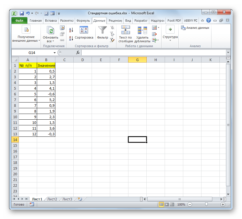
Выделяем ячейку, в которой будет выводиться итоговое значение стандартной ошибки, и клацаем по иконке «Вставить функцию».

Переход в Мастер функций в Microsoft Excel

Открывается Мастер функций. Производим перемещение в блок «Статистические». В представленном перечне наименований выбираем название «СТАНДОТКЛОН.В».

Переход в окно аргументов функции СТАНДОТКЛОН.В в Microsoft Excel

Запускается окно аргументов вышеуказанного оператора. СТАНДОТКЛОН.В предназначен для оценивания стандартного отклонения при выборке. Данный оператор имеет следующий синтаксис:
=СТАНДОТКЛОН.В(число1;число2;…)

«Число1» и последующие аргументы являются числовыми значениями или ссылками на ячейки и диапазоны листа, в которых они расположены. Всего может насчитываться до 255 аргументов этого типа. Обязательным является только первый аргумент.

Итак, устанавливаем курсор в поле «Число1». Далее, обязательно произведя зажим левой кнопки мыши, выделяем курсором весь диапазон выборки на листе. Координаты данного массива тут же отображаются в поле окна. После этого клацаем по кнопке «OK».

Окно аргументов функции СТАНДОТКЛОН.В в Microsoft Excel

В ячейку на листе выводится результат расчета оператора СТАНДОТКЛОН.В. Но это ещё не ошибка средней арифметической. Для того, чтобы получить искомое значение, нужно стандартное отклонение разделить на квадратный корень от количества элементов выборки. Для того, чтобы продолжить вычисления, выделяем ячейку, содержащую функцию СТАНДОТКЛОН.В. После этого устанавливаем курсор в строку формул и дописываем после уже существующего выражения знак деления (/). Вслед за этим клацаем по пиктограмме перевернутого вниз углом треугольника, которая располагается слева от строки формул. Открывается список недавно использованных функций. Если вы в нем найдете наименование оператора «КОРЕНЬ», то переходите по данному наименованию. В обратном случае жмите по пункту «Другие функции…».

Переход к дальнейшему продолжению написания формулы стандартной ошибки в Microsoft Excel

Снова происходит запуск Мастера функций. На этот раз нам следует посетить категорию «Математические». В представленном перечне выделяем название «КОРЕНЬ» и жмем на кнопку «OK».

Переход в окно аргументов функции КОРЕНЬ в Microsoft Excel

Открывается окно аргументов функции КОРЕНЬ. Единственной задачей данного оператора является вычисление квадратного корня из заданного числа. Его синтаксис предельно простой:
=КОРЕНЬ(число)

Как видим, функция имеет всего один аргумент «Число». Он может быть представлен числовым значением, ссылкой на ячейку, в которой оно содержится или другой функцией, вычисляющей это число. Последний вариант как раз и будет представлен в нашем примере.

Устанавливаем курсор в поле «Число» и кликаем по знакомому нам треугольнику, который вызывает список последних использованных функций. Ищем в нем наименование «СЧЁТ». Если находим, то кликаем по нему. В обратном случае, опять же, переходим по наименованию «Другие функции…».

Окно аргументов функции КОРЕНЬ в Microsoft Excel

В раскрывшемся окне Мастера функций производим перемещение в группу «Статистические». Там выделяем наименование «СЧЁТ» и выполняем клик по кнопке «OK».

Переход в окно аргументов функции СЧЁТ в Microsoft Excel

Запускается окно аргументов функции СЧЁТ. Указанный оператор предназначен для вычисления количества ячеек, которые заполнены числовыми значениями. В нашем случае он будет подсчитывать количество элементов выборки и сообщать результат «материнскому» оператору КОРЕНЬ. Синтаксис функции следующий:
=СЧЁТ(значение1;значение2;…)

В качестве аргументов «Значение», которых может насчитываться до 255 штук, выступают ссылки на диапазоны ячеек. Ставим курсор в поле «Значение1», зажимаем левую кнопку мыши и выделяем весь диапазон выборки. После того, как его координаты отобразились в поле, жмем на кнопку «OK».

Окно аргументов функции СЧЁТ в Microsoft Excel

После выполнения последнего действия будет не только рассчитано количество ячеек заполненных числами, но и вычислена ошибка средней арифметической, так как это был последний штрих в работе над данной формулой. Величина стандартной ошибки выведена в ту ячейку, где размещена сложная формула, общий вид которой в нашем случае следующий:
=СТАНДОТКЛОН.В(B2:B13)/КОРЕНЬ(СЧЁТ(B2:B13))

Результат вычисления ошибки средней арифметической составил 0,505793. Запомним это число и сравним с тем, которое получим при решении поставленной задачи следующим способом.

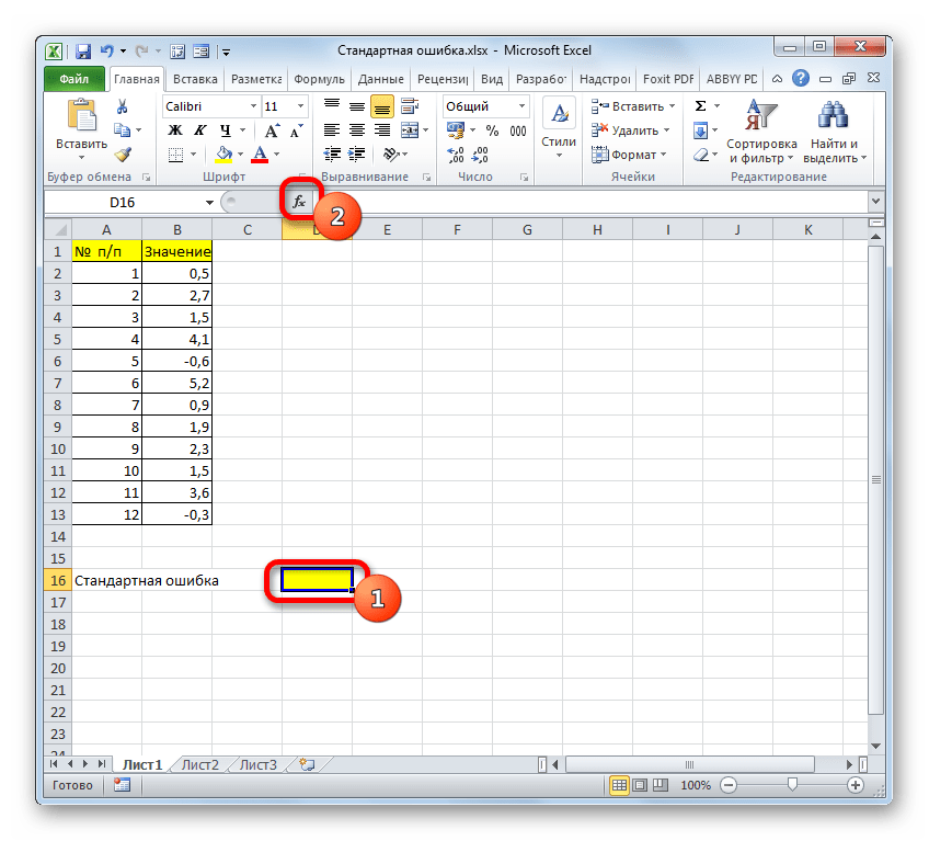
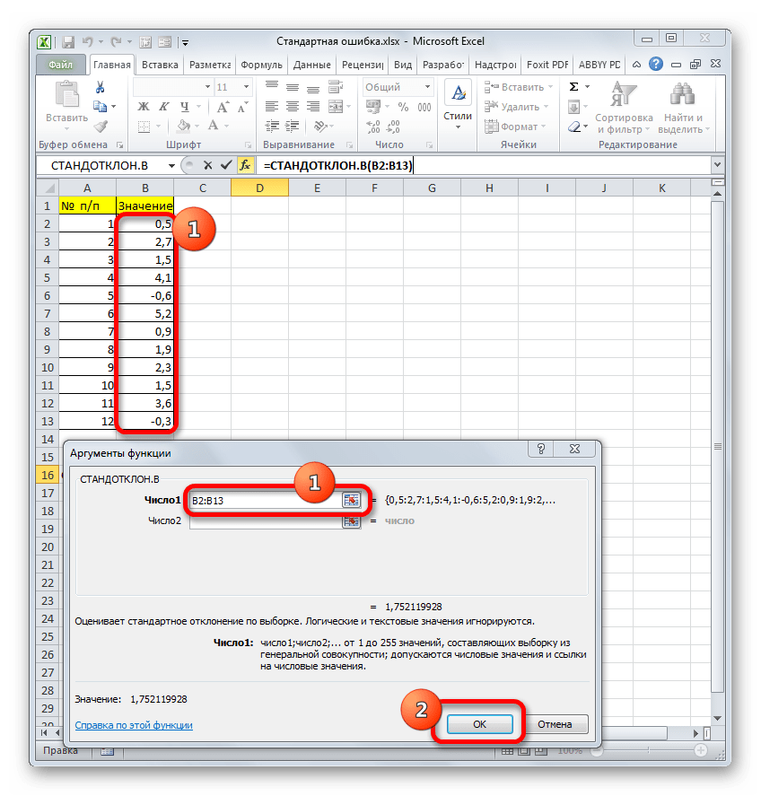
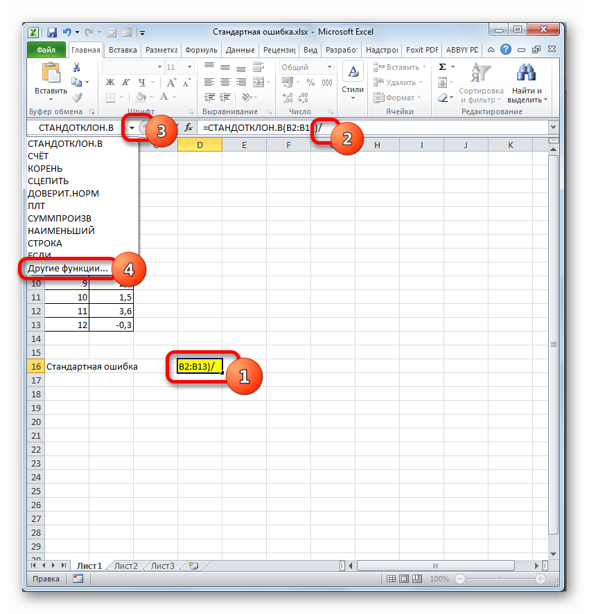
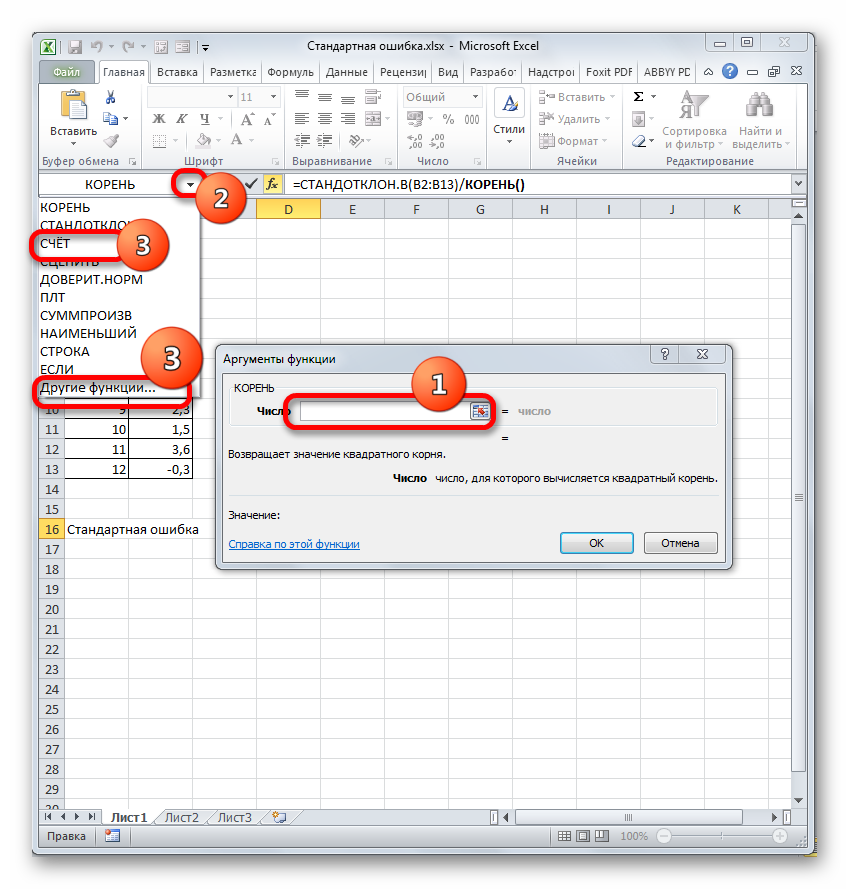
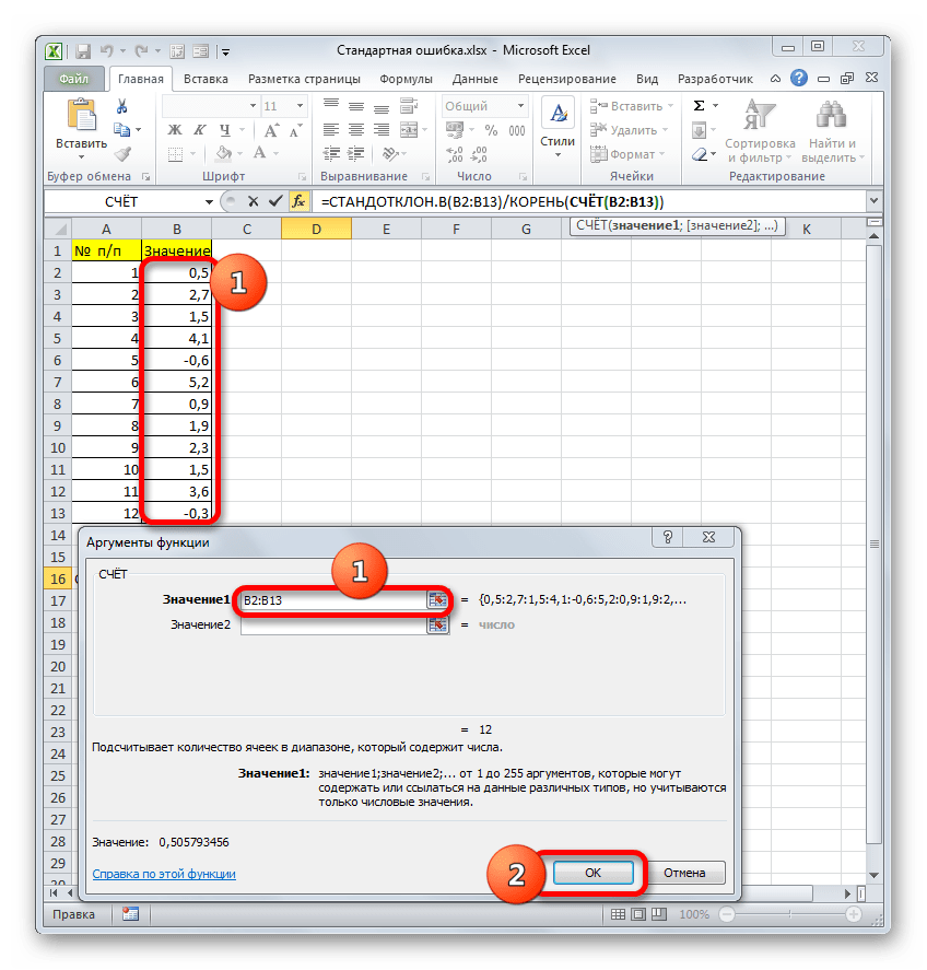
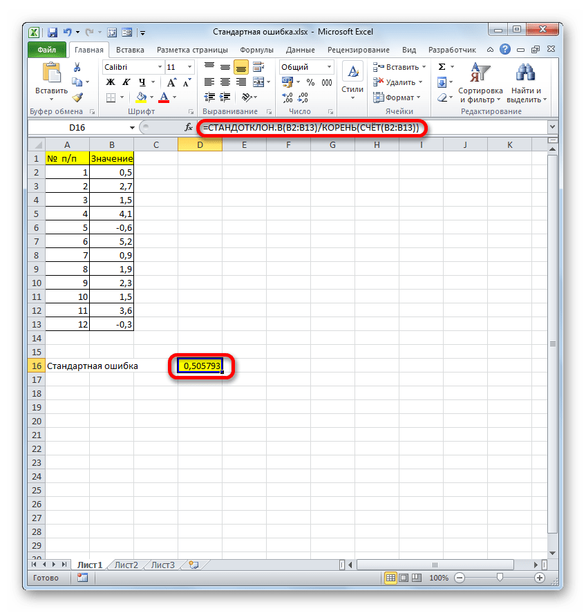
Результат вычисления стандартной ошибки в сложной формуле в Microsoft Excel

Но дело в том, что для малых выборок (до 30 единиц) для большей точности лучше применять немного измененную формулу. В ней величина стандартного отклонения делится не на квадратный корень от количества элементов выборки, а на квадратный корень от количества элементов выборки минус один. Таким образом, с учетом нюансов малой выборки наша формула приобретет следующий вид:

=СТАНДОТКЛОН.В(B2:B13)/КОРЕНЬ(СЧЁТ(B2:B13)-1)

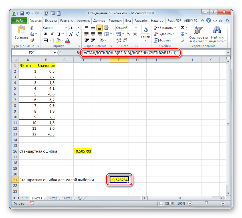
Результат вычисления стандартной ошибки для малой выборки в Microsoft Excel

Урок: Статистические функции в Экселе

Способ 2: применение инструмента «Описательная статистика»

Вторым вариантом, с помощью которого можно вычислить стандартную ошибку в Экселе, является применение инструмента «Описательная статистика», входящего в набор инструментов «Анализ данных» («Пакет анализа»). «Описательная статистика» проводит комплексный анализ выборки по различным критериям. Одним из них как раз и является нахождение ошибки средней арифметической.

Но чтобы воспользоваться данной возможностью, нужно сразу активировать «Пакет анализа», так как по умолчанию в Экселе он отключен.

После того, как открыт документ с выборкой, переходим во вкладку «Файл».

Переход во вкладку Файл в Microsoft Excel

Далее, воспользовавшись левым вертикальным меню, перемещаемся через его пункт в раздел «Параметры».

Перемещение в раздел Параметры в Microsoft Excel

Запускается окно параметров Эксель. В левой части данного окна размещено меню, через которое перемещаемся в подраздел «Надстройки».

Переход в подраздел надстройки окна параметров в Microsoft Excel

В самой нижней части появившегося окна расположено поле «Управление». Выставляем в нем параметр «Надстройки Excel» и жмем на кнопку «Перейти…» справа от него.

Переход в окно надстроек в Microsoft Excel

Запускается окно надстроек с перечнем доступных скриптов. Отмечаем галочкой наименование «Пакет анализа» и щелкаем по кнопке «OK» в правой части окошка.

Включение пакета анализа в окне надстроек в Microsoft Excel

После выполнения последнего действия на ленте появится новая группа инструментов, которая имеет наименование «Анализ». Чтобы перейти к ней, щелкаем по названию вкладки «Данные».

Переход во вкладку Данные в Microsoft Excel

После перехода жмем на кнопку «Анализ данных» в блоке инструментов «Анализ», который расположен в самом конце ленты.

Переход в Анализ данных в Microsoft Excel

Запускается окошко выбора инструмента анализа. Выделяем наименование «Описательная статистика» и жмем на кнопку «OK» справа.

Переход в описательную статистику в Microsoft Excel

Запускается окно настроек инструмента комплексного статистического анализа «Описательная статистика».
В поле «Входной интервал» необходимо указать диапазон ячеек таблицы, в которых находится анализируемая выборка. Вручную это делать неудобно, хотя и можно, поэтому ставим курсор в указанное поле и при зажатой левой кнопке мыши выделяем соответствующий массив данных на листе. Его координаты тут же отобразятся в поле окна.

В блоке «Группирование» оставляем настройки по умолчанию. То есть, переключатель должен стоять около пункта «По столбцам». Если это не так, то его следует переставить.

Галочку «Метки в первой строке» можно не устанавливать. Для решения нашего вопроса это не важно.

Далее переходим к блоку настроек «Параметры вывода». Здесь следует указать, куда именно будет выводиться результат расчета инструмента «Описательная статистика»:
- На новый лист;
- В новую книгу (другой файл);
- В указанный диапазон текущего листа.
Давайте выберем последний из этих вариантов. Для этого переставляем переключатель в позицию «Выходной интервал» и устанавливаем курсор в поле напротив данного параметра. После этого клацаем на листе по ячейке, которая станет верхним левым элементом массива вывода данных. Её координаты должны отобразиться в поле, в котором мы до этого устанавливали курсор.

Далее следует блок настроек определяющий, какие именно данные нужно вводить:
- Итоговая статистика;
- К-ый наибольший;
- К-ый наименьший;
- Уровень надежности.
Для определения стандартной ошибки обязательно нужно установить галочку около параметра «Итоговая статистика». Напротив остальных пунктов выставляем галочки на свое усмотрение. На решение нашей основной задачи это никак не повлияет.

После того, как все настройки в окне «Описательная статистика» установлены, щелкаем по кнопке «OK» в его правой части.

Окно описаительная статистика в Microsoft Excel

После этого инструмент «Описательная статистика» выводит результаты обработки выборки на текущий лист. Как видим, это довольно много разноплановых статистических показателей, но среди них есть и нужный нам – «Стандартная ошибка». Он равен числу 0,505793. Это в точности тот же результат, который мы достигли путем применения сложной формулы при описании предыдущего способа.

Результат расчета стандартной ошибки путем применения инструмента Описательная статистика в Microsoft Excel

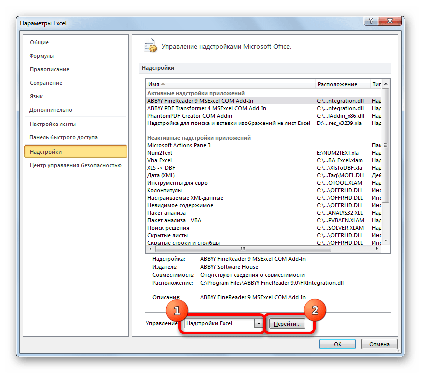
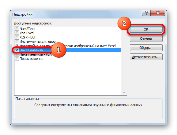
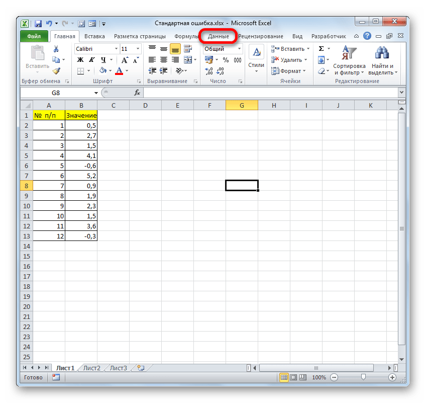
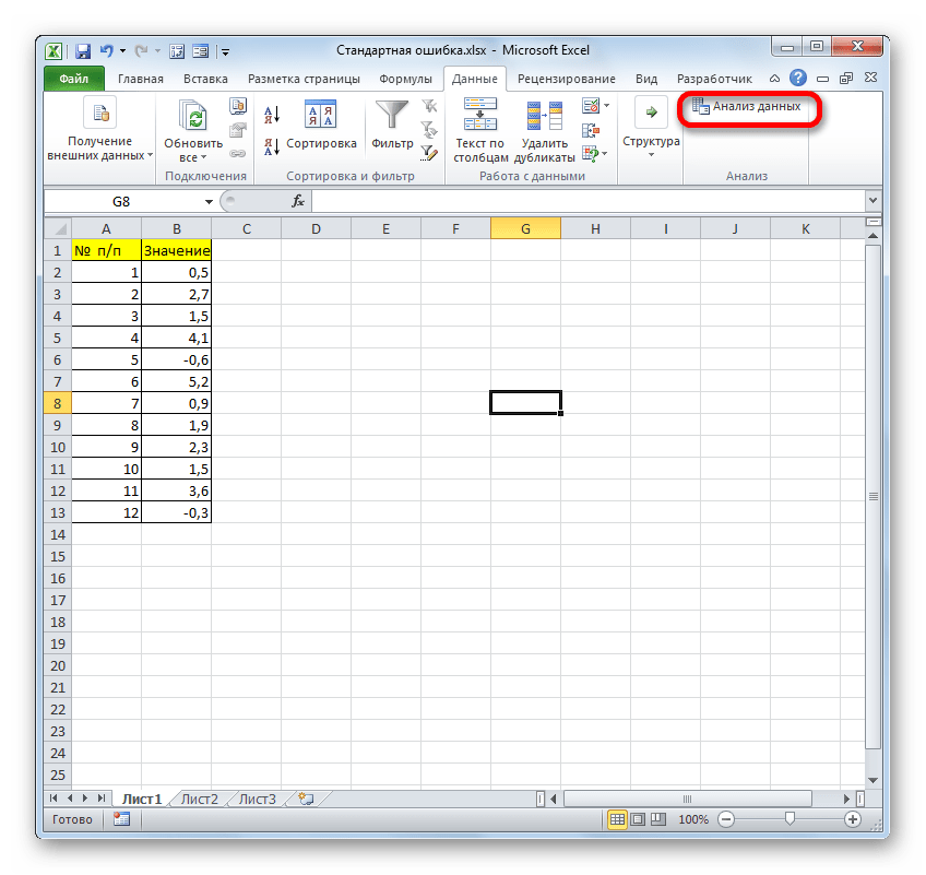
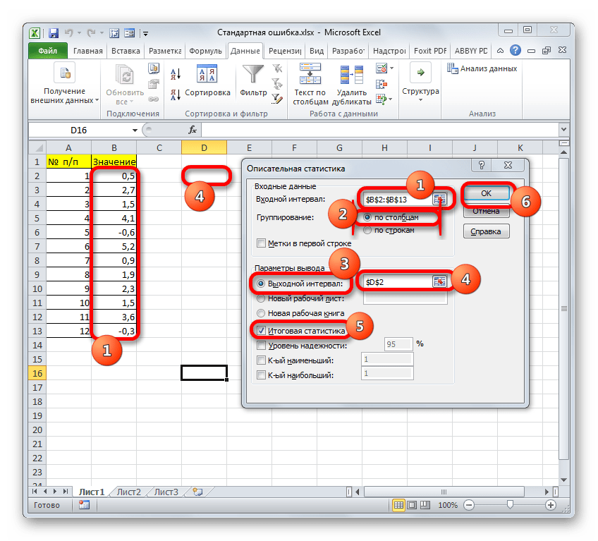
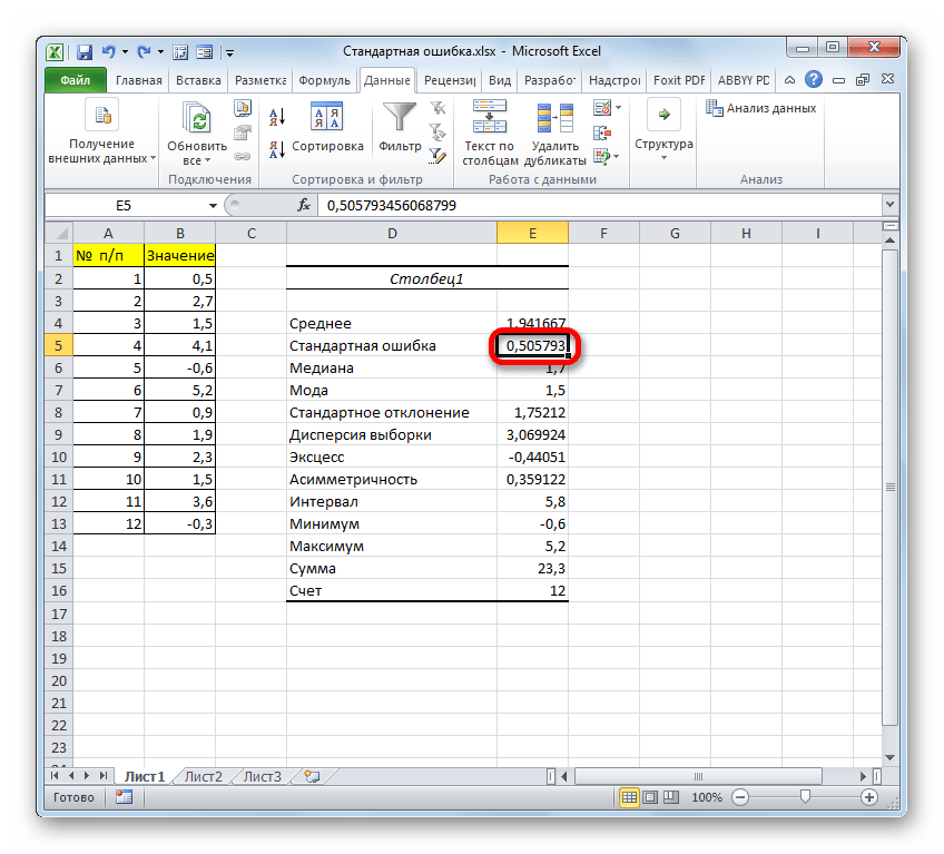
Урок: Описательная статистика в Экселе

Как видим, в Экселе можно произвести расчет стандартной ошибки двумя способами: применив набор функций и воспользовавшись инструментом пакета анализа «Описательная статистика». Итоговый результат будет абсолютно одинаковый. Поэтому выбор метода зависит от удобства пользователя и поставленной конкретной задачи. Например, если ошибка средней арифметической является только одним из многих статистических показателей выборки, которые нужно рассчитать, то удобнее воспользоваться инструментом «Описательная статистика». Но если вам нужно вычислить исключительно этот показатель, то во избежание нагромождения лишних данных лучше прибегнуть к сложной формуле. В этом случае результат расчета уместится в одной ячейке листа.

Источник

Основной задачей при управлении запасами является определение объема пополнения, то есть, сколько необходимо заказать поставщику. При расчете этого объема используется несколько параметров — сколько будет продано в будущем, за какое время происходит пополнение, какие остатки у нас на складе и какое количество уже заказано у поставщика. То, насколько правильно мы определим эти параметры, будет влиять на то, будет ли достаточно товара на складе или его будет слишком много. Но наибольшее влияние на эффективность управления запасами влияет то, насколько точен будет прогноз. Многие считают, что это вообще основной вопрос в управлении запасами. Действительно, точность прогнозирования очень важный параметр. Поэтому важно понимать, как его оценивать. Это важно и для выявления причин дефицитов или неликвидов, и при выборе программных продуктов для прогнозирования продаж и управления запасами.

В данной статье я представила несколько формул для расчета точности прогноза и ошибки прогнозирования. Кроме этого, вы сможете скачать файлы с примерами расчетов этого показателя.

Статистические методы

Для оценки прогноза продаж используются статистические оценки Оценка ошибки прогнозирования временного ряда. Самый простой показатель – отклонение факта от прогноза в количественном выражении.

В практике рассчитывают ошибку прогнозирования по каждой отдельной позиции, а также рассчитывают среднюю ошибку прогнозирования. Следующие распространенные показатели ошибки относятся именно к показателям средних ошибок прогнозирования.

К ним относятся:

MAPE – средняя абсолютная ошибка в процентах

где Z(t) – фактическое значение временного ряда, а – прогнозное.

Данная оценка применяется для временных рядов, фактические значения которых значительно больше 1. Например, оценки ошибки прогнозирования энергопотребления почти во всех статьях приводятся как значения MAPE.

Если же фактические значения временного ряда близки к 0, то в знаменателе окажется очень маленькое число, что сделает значение MAPE близким к бесконечности – это не совсем корректно. Например, фактическая цена РСВ = 0.01 руб/МВт.ч, a прогнозная = 10 руб/МВт.ч, тогда MAPE = (0.01 – 10)/0.01 = 999%, хотя в действительности мы не так уж сильно ошиблись, всего на 10 руб/МВт.ч. Для рядов, содержащих значения близкие к нулю, применяют следующую оценку ошибки прогноза.

MAE – средняя абсолютная ошибка

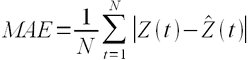Для оценки ошибки прогнозирования цен РСВ и индикатора БР корректнее использовать MAE.

После того, как получены значения для MAPE и/или MAE, то в работах обычно пишут: «Прогнозирование временного ряда энергопотребления с часовым разрешение проводилось на интервале с 01.01.2001 до 31.12.2001 (общее количество отсчетов N ~ 8500). Для данного прогноза значение MAPE = 1.5%». При этом, просматривая статьи, можно сложить общее впечатление об ошибки прогнозирования энергопотребления, для которого MAPE обычно колеблется от 1 до 5%; или ошибки прогнозирования цен на электроэнергию, для которого MAPE колеблется от 5 до 15% в зависимости от периода и рынка. Получив значение MAPE для собственного прогноза, вы можете оценить, насколько здорово у вас получается прогнозировать.

Кроме указанных методов иногда используют другие оценки ошибки, менее популярные, но также применимые. Подробнее об этих оценках ошибки прогноза читайте указанные статьи в Википедии.

ME – средняя ошибка

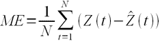
Встречается еще другое название этого показателя — Bias (англ. – смещение) демонстрирует величину отклонения, а также — в какую сторону прогноз продаж отклоняется от фактической потребности. Этот индикатор показывает, был ли прогноз оптимистичным или пессимистичным. То есть, отрицательное значение Bias говорит о том, что прогноз был завышен (реальная потребность оказалась ниже), и, наоборот, положительное значение о том, что прогноз был занижен. Цифровое значение показателя определяет величину отклонения (смещения).

MSE – среднеквадратичная ошибка

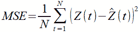RMSE – квадратный корень из среднеквадратичной ошибки

SD – стандартное отклонение

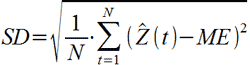
где ME – есть средняя ошибка, определенная по формуле выше.

Примечание. Примеры расчетов данных показателей представлены в файле Excel, который можно скачать, оставив электронный адрес в форме ниже. Скачать пример расчета в Excel >>>

Связь точности и ошибки прогнозирования

В начале этого обсуждения разберемся с определениями.

Ошибка прогноза — апостериорная величина отклонения прогноза от действительного состояния объекта. Если говорить о прогнозе продаж, то это показатель отклонения фактических продаж от прогноза.

Точность прогнозирования есть понятие прямо противоположное ошибке прогнозирования. Если ошибка прогнозирования велика, то точность мала и наоборот, если ошибка прогнозирования мала, то точность велика. По сути дела оценка ошибки прогноза MAPE есть обратная величина для точности прогнозирования — зависимость здесь простая.

Точность прогноза в % = 100% – MAPE, встречается еще название этого показателя Forecast Accuracy. Вы практически не найдете материалов о прогнозировании, в которых приведены оценки именно точности прогноза, хотя с точки зрения здравого маркетинга корректней говорить именно о высокой точности. В рекламных статьях всегда будет написано о высокой точности. Показатель точности прогноза выражается в процентах:

Если точность прогноза равна 100%, то выбранная модель описывает фактические значения на 100%, т.е. очень точно. Нужно сразу оговориться, что такого показателя никогда не будет, основное свойство прогноза в том, что он всегда ошибочен.
Если 0% или отрицательное число, то совсем не описывает, и данной модели доверять не стоит.

Выбрать подходящую модель прогноза можно с помощью расчета показателя точность прогноза. Модель прогноза, у которой показатель точность прогноза будет ближе к 100%, с большей вероятностью сделает более точный прогноз. Такую модель можно назвать оптимальной для выбранного временного ряда. Говоря о высокой точности, мы говорим о низкой ошибки прогноза и в этой области недопонимания быть не должно. Не имеет значения, что именно вы будете отслеживать, но важно, чтобы вы сравнивали модели прогнозирования или целевые показатели по одному показателю – ошибка прогноза или точность прогнозирования.

Ранее я использовала оценку MAPE, до тех пор пока не встретила формулу, которую рекомендует Валерий Разгуляев.

Примечание. Примеры расчетов данных показателей представлены в файле Excel, который можно скачать, оставив электронный адрес в форме. Скачать пример расчета в Excel >>>

Оценка ошибки прогноза – формула Валерия Разгуляева (сайт http://upravlenie-zapasami.ru/)

Одной из самых используемых формул оценки ошибки прогнозирования является следующая формула:

где: P – это прогноз, а S – факт за тот же месяц. Однако у этой формулы есть серьезное ограничение — как оценить ошибку, если факт равен нулю? Возможный ответ, что в таком случае D = 100% – который означает, что мы полностью ошиблись. Однако простой пример показывает, что такой ответ — не верен:

вариант	прогноз	факт	ошибка прогноза
№1	4	0	100%
№2	4	1	300%
№3	1	4	75%

Оказывается, что в варианте развития событий №2, когда мы лучше угадали спрос, чем в варианте №1, ошибка по данной формуле оказалась – больше. То есть ошиблась уже сама формула. Есть и другая проблема, если мы посмотрим на варианты №2 и №3, то увидим, что имеем дело с зеркальной ситуацией в прогнозе и факте, а ошибка при этом отличается – в разы!.. То есть при такой оценке ошибки прогноза нам лучше его заведомо делать менее точным, занижая показатель – тогда ошибка будет меньше!.. Хотя понятно, что чем точнее будет прогноз – тем лучше будет и закупка. Поэтому для расчёта ошибки Валерий Разгуляев рекомендует использовать следующую формулу:

В таком случае для тех же примеров ошибка рассчитается иначе:

вариант	прогноз	факт	ошибка прогноза
№1	4	0	100%
№2	4	1	75%
№3	1	4	75%

Как мы видим, в варианте №1 ошибка становится равной 100%, причём это уже – не наше предположение, а чистый расчёт, который можно доверить машине. Зеркальные же варианты №2 и №3 – имеют и одинаковую ошибку, причём эта ошибка меньше ошибки самого плохого варианта №1. Единственная ситуация, когда данная формула не сможет дать однозначный ответ – это равенство знаменателя нулю. Но максимум из прогноза и факта равен нулю, только когда они оба равны нулю. В таком случае получается, что мы спрогнозировали отсутствие спроса, и его, действительно, не было – то есть ошибка тоже равна нулю – мы сделали совершенно точное предсказание.

Визуальный метод – графический

Визуальный метод состоит в том, что мы на график выводим значение прогнозной модели и факта продаж по тем моделям, которые хотим сравнить. Далее сравниваем визуально, насколько прогнозная модель близка к фактическим продажам. Давайте рассмотрим на примере. В таблице представлены две прогнозные модели, а также фактические продажи по этому товару за тот же период. Для наглядности мы также рассчитали ошибку прогнозирования по обеим моделям.

По графикам очевидно, что модель 2 описывает лучше продажи этого товара. Оценка ошибки прогнозирования тоже это показывает – 65% и 31% ошибка прогнозирования по модели 1 и модели 2 соответственно.

Недостатком данного метода является то, что небольшую разницу между моделями сложно выявить — разницу в несколько процентов сложно оценить по диаграмме. Однако эти несколько процентов могут существенно улучшить качество прогнозирования и планирования пополнения запасов в целом.

Использование формул ошибки прогнозирования на практике

Практический аспект оценки ошибки прогнозирования я вывела отдельным пунктом. Это связано с тем, что все статистические методы расчета показателя ошибки прогнозирования рассчитывают то, насколько мы ошиблись в прогнозе в количественных показателях. Давайте теперь обсудим, насколько такой показатель будет полезен в вопросах управления запасами. Дело в том, что основная цель управления запасами — обеспечить продажи, спрос наших клиентов. И, в конечном счете, максимизировать доход и прибыль компании. А эти показатели оцениваются как раз в стоимостном выражении. Таким образом, нам важно при оценке ошибки прогнозирования понимать какой вклад каждая позиция внесла в объем продаж в стоимостном выражении. Когда мы оцениваем ошибку прогнозирования в количественном выражении мы предполагаем, что каждый товар имеет одинаковый вес в общем объеме продаж, но на самом деле это не так – есть очень дорогие товары, есть товары, которые продаются в большом количестве, наша группа А, а есть не очень дорогие товары, есть товары которые вносят небольшой вклад в объем продаж. Другими словами большая ошибка прогнозирования по товарам группы А будет нам «стоить» дороже, чем низкая ошибка прогнозирования по товарам группы С, например. Для того, чтобы наша оценка ошибки прогнозирования была корректной, релевантной целям управления запасами, нам необходимо оценивать ошибку прогнозирования по всем товарам или по отдельной группе не по средними показателями, а средневзвешенными с учетом прогноза и факта в стоимостном выражении.

Пример расчета такой оценки Вы сможете увидеть в файле Excel.

При этом нужно помнить, что для оценки ошибки прогнозирования по отдельным позициям мы рассчитываем по количеству, но вот если нам важно понять в целом ошибку прогнозирования по компании, например, для оценки модели, которую используем, то нам нужно рассчитывать не среднюю оценку по всем товарам, а средневзвешенную с учетом стоимостной оценки. Оценку можно брать по ценам себестоимости или ценам продажи, это не играет большой роли, главное, эти же цены (тип цен) использовать при всех расчетах.

Для чего используется ошибка прогнозирования

В первую очередь, оценка ошибки прогнозирования нам необходима для оценки того, насколько мы ошибаемся при планировании продаж, а значит при планировании поставок товаров. Если мы все время прогнозируем продажи значительно больше, чем потом фактически продаем, то вероятнее всего у нас будет излишки товаров, и это невыгодно компании. В случае, когда мы ошибаемся в обратную сторону – прогнозируем продажи меньше чем фактические продажи, с большой вероятностью у нас будут дефициты и компания не дополучит прибыль. В этом случае ошибка прогнозирования служит индикатором качества планирования и качества управления запасами.

Индикатором того, что повышение эффективности возможно за счет улучшения качества прогнозирования. За счет чего можно улучшить качество прогнозирования мы не будем здесь рассматривать, но одним из вариантов является поиск другой модели прогнозирования, изменения параметров расчета, но вот насколько новая модель будет лучше, как раз поможет показатель ошибки прогнозирования или точности прогноза. Сравнение этих показателей по нескольким моделям поможет определить ту модель, которая дает лучше результат.

В идеальном случае, мы можем так подбирать модель для каждой отдельной позиции. В этом случае мы будем рассчитывать прогноз по разным товарам по разным моделям, по тем, которые дают наилучший вариант именно для конкретного товара.

Также этот показатель можно использовать при выборе автоматизированного инструмента для прогнозирования спроса и управления запасами. Вы можете сделать тестовые расчеты прогноза в предлагаемой программе и сравнить ошибку прогнозирования полученного прогноза с той, которая есть у вашей существующей модели. Если у предлагаемого инструмента ошибка прогнозирования меньше. Значит, этот инструмент можно рассматривать для применения в компании. Кроме этого, показатель точности прогноза или ошибки прогнозирования можно использовать как KPI сотрудников, которые отвечают за подготовку прогноза продаж или менеджеров по закупкам, в том случае, если они рассчитывают прогноз будущих продаж при расчете заказа.

Если вы хотите повысить эффективность управления запасами и увеличить оборачиваемость товарных запасов, предлагаю изучить мастер-класс «Как увеличить оборачиваемость товарных запасов».

Источник: сайт http://uppravuk.net/

Источник

Стандартная ошибка предсказания это

2.3 Прогнозирование величины y

Что такое стандартная ошибка оценки? (Определение и пример)

Пример: стандартная ошибка оценки в Excel

Дополнительные ресурсы

MPE — Mean Percent Error

MAPE — Mean Absolute Percent Error

WMAPE / MAD-Mean Ratio / WAPE — Weighted Absolute Percent Error

RMSE (as %) / nRMSE — Root Mean Square Error

MASE — Mean Absolute Scaled Error

Об авторе

HeinzBr

Correlation and Regression

The Standard Error of Estimate: How Large Are the Prediction Errors?

Standard Error of Estimate

Detection of a Trend in Population Estimates

5.2 VARIANCE COMPONENTS

Example 5.1 Population Size, Estimates, Standard Error of the Estimates, and Confidence Intervals for Owl Pairs in Fig. 5.3

Multiple Regression

Typical Prediction Error: Standard Error of Estimate

Multiple Regression

Confidence Intervals for the Coefficients

Multiple Regression

Confidence Intervals for the Coefficients

Simple Regression

Abstract

Bootstrap Method

Approximating Standard Error of a Sample Estimate

Pearson, Karl

The Biometric School

Correlation and Regression

The Standard Error of Estimate: How Large Are the Prediction Errors?

Standard Error of Estimate

Detection of a Trend in Population Estimates

5.2 VARIANCE COMPONENTS

Example 5.1 Population Size, Estimates, Standard Error of the Estimates, and Confidence Intervals for Owl Pairs in Fig. 5.3

Multiple Regression

Typical Prediction Error: Standard Error of Estimate

Multiple Regression

Confidence Intervals for the Coefficients

Multiple Regression

Confidence Intervals for the Coefficients

Simple Regression

Abstract

Bootstrap Method

Approximating Standard Error of a Sample Estimate

Pearson, Karl

The Biometric School

Расчет ошибки средней арифметической

Способ 1: расчет с помощью комбинации функций

Способ 2: применение инструмента «Описательная статистика»

ME – средняя ошибка

А вот еще интересные материалы: