Площадь под ROC-кривой – один из самых популярных функционалов качества в задачах бинарной классификации. На мой взгляд, простых и полных источников информации «что же это такое» нет. Как правило, объяснение начинают с введения разных терминов (FPR, TPR), которые нормальный человек тут же забывает. Также нет разборов каких-то конкретных задач по AUC ROC. В этом посте описано, как я объясняю эту тему студентам и своим сотрудникам…

Допустим, решается задача классификации с двумя классами {0, 1}. Алгоритм выдаёт некоторую оценку (может, но не обязательно, вероятность) принадлежности объекта к классу 1. Можно считать, что оценка принадлежит отрезку [0, 1].
Часто результат работы алгоритма на фиксированной тестовой выборке визуализируют с помощью ROC-кривой (ROC = receiver operating characteristic, иногда говорят «кривая ошибок»), а качество оценивают как площадь под этой кривой – AUC (AUC = area under the curve). Покажем на конкретном примере, как строится кривая.
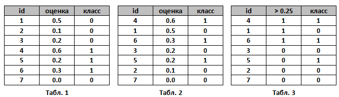
Пусть алгоритм выдал оценки, как показано в табл. 1. Упорядочим строки табл. 1 по убыванию ответов алгоритма – получим табл. 2. Ясно, что в идеале её столбец «класс» тоже станет упорядочен (сначала идут 1, потом 0); в самом худшем случае – порядок будет обратный (сначала 0, потом 1); в случае «слепого угадывания» будет случайное распределение 0 и 1.
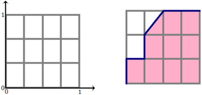
Чтобы нарисовать ROC-кривую, надо взять единичный квадрат на координатной плоскости, см. рис. 1, разбить его на m равных частей горизонтальными линиями и на n – вертикальными, где m – число 1 среди правильных меток теста (в нашем примере m=3), n – число нулей (n=4). В результате квадрат разбивается сеткой на m×n блоков.
Теперь будем просматривать строки табл. 2 сверху вниз и прорисовывать на сетке линии, переходя их одного узла в другой. Стартуем из точки (0, 0). Если значение метки класса в просматриваемой строке 1, то делаем шаг вверх; если 0, то делаем шаг вправо. Ясно, что в итоге мы попадём в точку (1, 1), т.к. сделаем в сумме m шагов вверх и n шагов вправо.
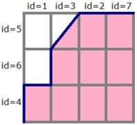
На рис. 1 (справа) показан путь для нашего примера – это и является ROC-кривой. Важный момент: если у нескольких объектов значения оценок равны, то мы делаем шаг в точку, которая на a блоков выше и b блоков правее, где a – число единиц в группе объектов с одним значением метки, b – число нулей в ней. В частности, если все объекты имеют одинаковую метку, то мы сразу шагаем из точки (0, 0) в точку (1, 1).
AUC ROC – площадь под ROC-кривой – часто используют для оценивания качества упорядочивания алгоритмом объектов двух классов. Ясно, что это значение лежит на отрезке [0, 1]. В нашем примере AUC ROC = 9.5 / 12 ~ 0.79.
Выше мы описали случаи идеального, наихудшего и случайного следования меток в упорядоченной таблице. Идеальному соответствует ROC-кривая, проходящая через точку (0, 1), площадь под ней равна 1. Наихудшему – ROC-кривая, проходящая через точку (1, 0), площадь под ней – 0. Случайному – что-то похожее на диагональ квадрата, площадь примерно равна 0.5.

Замечание. ROC-кривая считается неопределённой для тестовой выборки целиком состоящей из объектов только одного класса. Большинство современных реализаций выдают ошибку при попытки построить её в этом случае
Сетка на рис. 1 разбила квадрат на m×n блоков. Ровно столько же пар вида (объект класса 1, объект класса 0), составленных из объектов тестовой выборки. Каждый закрашенный блок на рис. 1 соответствует паре (объект класса 1, объект класса 0), для которой наш алгоритм правильно предсказал порядок (объект класса 1 получил оценку выше, чем объект класса 0), незакрашенный блок – паре, на которой ошибся.
Таким образом, AUC ROC равен доле пар объектов вида (объект класса 1, объект класса 0), которые алгоритм верно упорядочил, т.е. первый объект идёт в упорядоченном списке раньше. Численно это можно записать так:

Замечание. В формуле (*) все постоянно ошибаются, забывая случай равенства ответов алгоритма на нескольких объектах. Также эту формулу все постоянно переоткрывают. Она хороша тем, что легко обобщается и на другие задачи обучения с учителем.
Принятие решений на основе ROC-кривой
Пока наш алгоритм выдавал оценки принадлежности к классу 1. Ясно, что на практике нам часто надо будет решить: какие объекты отнести к классу 1, а какие к классу 0. Для этого нужно будет выбрать некоторый порог (объекты с оценками выше порога считаем принадлежащими классу 1, остальные – 0).
Выбору порога соответствует выбор точки на ROC-кривой. Например, для порога 0.25 и нашего примера – точка указана на рис. 4 (1/4, 2/3). см. табл. 3
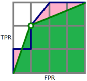
Заметим, что 1/4 – это процент точек класса 0, которые неверно классифицированы нашим алгоритмом (это называется FPR = False Positive Rate), 2/3 – процент точек класса 1, которые верно классифицированы нашим алгоритмом (это называется TPR = True Positive Rate). Именно в этих координатах (FPR, TPR) построена ROC-кривая. Часто в литературе её определяют как кривую зависимости TPR от FPR при варьировании порога для бинаризации.
Кстати, для бинарных ответов алгоритма тоже можно вычислить AUC ROC, правда это практически никогда не делают, поскольку ROC-кривая состоит из трёх точек, соединёнными линиями: (0,0), (FPR, TPR), (1, 1), где FPR и TPR соответствуют любому порогу из интервала (0, 1). На рис. 4 (зелёным) показана ROC-кривая бинаризованного решения, заметим, что AUC после бинаризации уменьшился и стал равным 8.5/12 ~ 0.71.

В общем случае, как видно из рис. 5 AUC ROC для бинарного решения равна

(как сумма площадей двух треугольников и квадрата). Это выражение имеет самостоятельную ценность и является «честной точностью» в задаче с дисбалансом классов (но об этом надо писать отдельный пост).
Задача
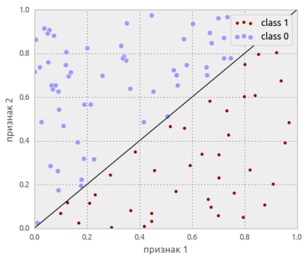
На ответах алгоритма a(x) объекты класса 0 распределены с плотностью p(a)=2-2a, а объекты класса 1 – с плотностью p(a)=2a, см. рис. 6. Интуитивно понятно, что алгоритм обладает некоторой разделяющей способностью (большинство объектов класса 0 имеют оценку меньше 0.5, а большинство объектов класса 1 – больше). Попробуйте угадать, чему здесь равен AUC ROC, а мы покажем как построить ROC-кривую и вычислить площадь под ней. Отметим, что здесь мы не работаем с конкретной тестовой выборкой, а считаем, что знаем распределения объектов всех классов. Такое может быть, например, в модельной задаче, когда объекты лежат в единичном квадрате, объекты выше одной из диагоналей принадлежат классу 0, ниже – классу 1, для решения используется логистическая регрессия (см. рис. 7). В случае, когда решение зависит только от одного признака (при втором коэффициент равен нулю), получаем как раз ситуацию, описанную в нашей задаче.

Значение TPR при выборе порога бинаризации равно площади, изображённой на рис. 6 (центр), а FPR – площади, изображённой на рис. 6 (справа), т.е.

Параметрическое уравнение для ROC-кривой получено, можно уже сразу вычислить площадь под ней:

Но если Вы не любите параметрическую запись, легко получить:

Заметим, что максимальная точность достигается при пороге бинаризации 0.5 (почему?), и она равна 3/4 = 0.75 (что не кажется очень большой). Это частая ситуация: AUC ROC существенно выше максимальной достижимой точности (accuracy)!
Кстати, AUC ROC бинаризованного решения (при пороге бинаризации 0.5) равна 0.75! Подумайте, почему это значение совпало с точностью?
В такой «непрерывной» постановке задачи (когда объекты двух классов описываются плотностями) AUC ROC имеет вероятностный смысл: это вероятность того, что случайно взятый объект класса 1 имеет оценку принадлежности к классу 1 выше, чем случайно взятый объект класса 0.

Для нашей модельной задачи можно провести несколько экспериментов: взять конечные выборки разной мощности с указанными распределениями. На рис. 8 показаны значения AUC ROC в таких экспериментах: все они распределены около теоретического значения 5/6, но разброс достаточно велик для небольших выборок. Запомните: для оценки AUC ROC выборка в несколько сотен объектов мала!

Также полезно посмотреть, как выглядят ROC-кривые в наших экспериментах. Естественно, при увеличении объёма выборок ROC-кривые, построенные по выборкам, будут сходиться к теоретической кривой (построенной для распределений).

Замечание
Интересно, что в рассмотренной задаче исходные данные линейны (например, плотности – линейные функции), а ответ (ROC-кривая) нелинейная (и даже неполиномиальная) функция!
Замечание
Почему-то многие считают, что ROC-кривая всегда является ступенчатой функцией – лишь при построении её для конечной выборки, в которой нет объектов с одинаковыми оценками. Полезно посмотреть на интерактивную визуализацию ROC-кривых для нормально распределённых классов.
Максимизация AUC ROC на практике
Оптимизировать AUC ROC напрямую затруднительно по нескольким причинам:
- эта функция недифференцируема по параметрам алгоритма,
- она в явном виде не разбивается на отдельные слагаемые, которые зависят от ответа только на одном объекте (как происходит в случае log_loss).
Есть несколько подходов к оптимизации
- замена в (*) индикаторной функции на похожую дифференцируемую функцию,
- использование смысла функционала (если это вероятность верного упорядочивания пары объектов, то можно перейти к новой выборке, состоящей из пар),
- ансамблирование нескольких алгоритмов с преобразованием их оценок в ранги (логика здесь простая: AUC ROC зависит только от порядка объектов, поэтому конкретные оценки не должны существенно влиять на ответ).
Замечания
- AUC ROC не зависит от строго возрастающего преобразования ответов алгоритма (например, возведения в квадрат), поскольку зависит не от самих ответов, а от меток классов объектов при упорядочивании по этим ответам.
- Часто используют критерий качества Gini, он принимает значение на отрезке [–1, +1] и линейно выражается через площадь под кривой ошибок:
Gini = 2 ×AUC_ROC – 1
- AUC ROC можно использовать для оценки качества признаков. Считаем, что значения признака — это ответы нашего алгоритма (не обязательно они должны быть нормированы на отрезок [0, 1], ведь нам важен порядок). Тогда выражение 2×|AUC_ROC — 0.5| вполне подойдёт для оценки качества признака: оно максимально, если по этому признаку 2 класса строго разделяются и минимально, если они «перемешаны».
- Практически во всех источниках приводится неверный алгоритм построения ROC-кривой и вычисления AUC ROC. По нашему описанию легко эти алгоритмы исправить…
- Часто утверждается, что AUC ROC не годится для задач с сильным дисбалансом классов. При этом приводятся совершенно некорректные обоснования этого. Рассмотрим одно из них. Пусть в задаче 1 000 000 объектов, при этом только 10 объектов из первого класса. Допустим, что объекты это сайты интернета, а первый класс – сайты, релевантные некоторому запросу. Рассмотрим алгоритм, ранжирующий все сайты в соответствии в эти запросом. Пусть он в начало списка поставил 100 объектов класса 0, потом 10 – класса 1, потом – все остальные класса 0. AUC ROC будет довольно высоким: 0.9999. При этом ответ алгоритма (если, например, это выдача поисковика) нельзя считать хорошей: в верхней части выдачи 100 нерелевантных сайтов. Разумеется, нам не хватит терпения пролистать выдачу и добраться до 10 тех самых релевантных.
В чём некорректность этого примера?! Главное: в том, что он никак не использует дисбаланс классов. С таким же успехом объектов класса 1 могло быть 500 000 – ровно половина, тогда AUC ROC чуть поменьше: 0.9998, но суть остаётся прежней. Таким образом, этот пример не показывает неприменимость AUC ROC в задачах с дисбалансом классов, а лишь в задачах поиска! Для таких задач есть другие функционалы качества, кроме того, есть специальные вариации AUC, например AUC@k. - В банковском скоринге AUC_ROC очень популярный функционал, хотя очевидно, что он также здесь не очень подходит. Банк может выдать ограниченное число кредитов, поэтому главное требование к алгоритму – чтобы среди объектов, которые получили наименьшие оценки были только представители класса 0 («вернёт кредит», если мы считаем, что класс 1 – «не вернёт» и алгоритм оценивает вероятность невозврата). Об этом можно судить по форме ROC-кривой (см. рис. 10).

П.С.
Если Вы дочитали до конца — можете попробовать пройти тест по AUC ROC (авторский, публикуется впервые). Задачи теста можно обсуждать в комментариях. Любые замечание по тексту — смело пишите!
Что можно ещё почитать…
- Wiki (и там есть хорошие ссылки!)
- Логистическая регрессия и ROC-анализ — математический аппарат
- Задачки про AUC (ROC)
Материал из MachineLearning.
(Перенаправлено с ROC-кривая)
Перейти к: навигация, поиск
Содержание
- 1 Задача классификации
- 2 TPR и FPR
- 3 ROC-кривая
- 4 Площадь под ROC-кривой AUC
- 5 Алгоритм построения ROC-кривой
- 6 Чувствительность и специфичность
- 7 История
- 8 См. также
- 9 Ссылки
Кривая ошибок или ROC-кривая – графичекая характеристика качества бинарного классификатора, зависимость доли верных положительных классификаций от доли ложных положительных классификаций при варьировании порога решающего правила. Преимуществом ROC-кривой является её инвариантность относительно отношения цены ошибки I и II рода.
Задача классификации
Рассмотрим задачу классификации в случае двух классов, называемых «положительным» и «отрицательным». Обозначим множество классов через . Большинство известных классификаторов могут быть представлены в виде
где
— произвольный объект,
— дискриминантная функция,
— вектор параметров, определяемый по обучающей выборке,
— порог.
Уравнение определяет разделяющую поверхность.
Примером является линейный классификатор, в котором дискриминантная функция имеет вид скалярного произведения вектора описания объекта на вектор параметров:
.
Пусть – цена ошибки (штраф за ошибку) на объекте класса
.
Для байесовского классификатора при достаточно общих предположениях доказано, что оптимальное значение порога зависит только от соотношения цены ошибок:
тогда как оптимальное значение вектора параметров , наоборот, зависит от выборки и не зависит от цены ошибок.
Таким образом, варьирование порога для многих классификаторов эквивалентно варьированию отношения цены ошибок на отрицательных и положительных объектах.
На практике цены ошибок зависят от особенностей конкретной задачи (например, от различных экономических соображений или экспертных оценок) и могут многократно пересматриваться.
Заметим, что частным случаем линейного байесовского классификатора является логистическая регрессия.
ROC-кривая наглядно представляет, каким будет качество классификации при различных и фиксированном
.
TPR и FPR
Пусть задана выборка объектов с соответствующими им верными ответами
.
Тогда для классификатора можно определить две характеристики качества:
- Доля ложных положительных классификаций (False Positive Rate, FPR):
- Доля верных положительных классификаций (True Positive Rate, TPR):
ROC-кривая
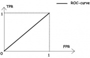

Рис.1. «Случайное гадание».
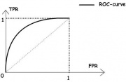
Рис.2. «Хороший» классификатор.
ROC-кривая показывает зависимость TPR от FPR при варьировании порога .
Она проходит из точки , соответствующей максимальному значению
, в точку
, соответствующую минимальному значению
.
При все объекты классифицируются как отрицательные, и ошибки возникают на всех положительных объектах,
,
.
При все объекты классифицируются как положительные, и ошибки возникают на всех отрицательных объектах,
,
.
ROC-кривая монотонно не убывает.
Чем выше лежит кривая, тем лучше качество классификации.
На рисунке 1 приведена ROC-кривая, соответствующая худшему случаю — алгоритму «случайного гадания».
На рисунке 2 изображён общий случай.
Лучший случай — это кривая, проходящая через точки
ROC-кривая может быть вычислена по любой выборке. Однако ROC-кривая, вычисленная по обучающей выборке, является оптимистично смещённой влево-вверх вследствие переобучения. Величину этого смещения предсказать довольно трудно, поэтому на практике ROC-кривую всегда оценивают по независомой тестовой выборке.
Площадь под ROC-кривой AUC
Площадь под ROC-кривой AUC (Area Under Curve) является агрегированной характеристикой качества классификации, не зависящей от соотношения цен ошибок.
Чем больше значение AUC, тем «лучше» модель классификации.
Данный показатель часто используется для сравнительного анализа нескольких моделей классификации.
Алгоритм построения ROC-кривой
Следующий алгоритм строит ROC-кривую за обращений к дискриминантной функции.
Входные данные:
Результат:
1. вычислить количество представителей классови
в выборке:
; 2. упорядочить выборку
по убыванию значений
; 3. установить начальную точку ROC-кривой:
;
; 4. для всех
если
, то сместиться на один шаг вправо:
;
; 5. иначе сместиться на один шаг вверх:
;
Чувствительность и специфичность
Наряду с FPR и TPR используют также показатели чувствительности и специфичности, которые также изменяются в интервале :
Модель с высокой чувствительностью часто дает истинный результат при наличии положительного исхода (обнаруживает положительные примеры). Наоборот, модель с высокой специфичностью чаще дает истинный результат при наличии отрицательного исхода (обнаруживает отрицательные примеры). Если рассуждать в терминах медицинской диагностики, где модель классификации пациентов на больных и здоровых называется диагностическим тестом, то получится следующее:
- чувствительный диагностический тест проявляется в гипердиагностике – максимальном предотвращении пропуска больных;
- специфичный диагностический тест диагностирует только доподлинно больных. Это важно в случае, когда, например, лечение больного связано с серьезными побочными эффектами и гипердиагностика пациентов нежелательна.
История
Термин операционная характеристика приёмника (Receiver Operating Characteristic, ROC) пришёл из теории обработки сигналов.
Эту характеристику впервые ввели во время II мировой войны, после поражения американского военного флота в Пёрл Харборе в 1941 году, когда была осознана проблема повышения точности распознавания самолётов противника по радиолокационному сигналу. Позже нашлись и другие применения: медицинская диагностика, приёмочный контроль качества, кредитный скоринг, предсказание лояльности клиентов, и т.д.
См. также
- Линейный классификатор
- Логистическая регрессия
Ссылки
- Логистическая регрессия и ROC-анализ
- RoC-curve (english wikipedia)
Площадь под ROC-кривой (Area Under Curve – площадь под кривой, Receiver Operating Characteristic – рабочая характеристика приёмника) – это метрика оценки для задач Бинарной классификации (Binary Classification). Площадь под кривой (AUC) является мерой способности классификатора различать классы и используется в качестве сводки кривой ROC:

Представьте: вы создали свою Модель (Model) Машинного обучения (ML), но что же дальше? Вам необходимо оценить ее и оценить качество, чтобы затем Вы могли решить, стоит ли она внедрения. Вот тут-то и пригодится кривая AUC ROC.
Название может показаться скучным, но оно просто говорит о том, что мы вычисляем «Площадь под кривой» (AUC) «рабочей характеристики приёмника (ROC). Пока много неясного, но мы подробно рассмотрим, что означают эти термины, и все встанет на свои места.
ROC-кривая помогает визуализировать, насколько хорошо работает классификатор машинного обучения. Хотя она работает только для задач двоичной классификации, ближе к концу мы увидим, как расширить его, чтобы решать проблемы Мультиклассовой классификации (Multi-Class Classification).
Мы также затронем такие темы, как Чувствительность (Sensitivity) и Специфичность (Specificity), поскольку это ключевые вспомогательные термины.
Матрица ошибок
Из Матрицы ошибок (Confusion Matrix) мы можем вывести некоторые важные показатели. Это показатель успешности классификации, где классов два или более. Это таблица с 4 различными комбинациями сочетаний прогнозируемых и фактических значений.

Давайте рассмотрим значения ячеек (истинно позитивные, ошибочно позитивные, ошибочно негативные, истинно негативные) с помощью «беременной» аналогии.

Истинно позитивное предсказание (True Positive, сокр. TP)
Вы предсказали положительный результат, и женщина действительно беременна.
Истинно отрицательное предсказание (True Negative, TN)
Вы предсказали отрицательный результат, и мужчина действительно не беременен.
Ошибочно положительное предсказание (ошибка типа I, False Positive, FN)
Вы предсказали положительный результат (мужчина беременен), но на самом деле это не так.
Ошибочно отрицательное предсказание (ошибка типа II, False Negative, FN)
Вы предсказали, что женщина не беременна, но на самом деле она беременна.
Чувствительность
Очевидно, желательны более высокий уровень TP и более низкий уровень FN. Чувствительность говорит нам, какая часть положительного класса была правильно классифицирована:
$$Чувствительность = frac{TP}{TP + FN}$$
$$TPspace{}{–}space{количество}space{истинно}space{позитивных}space{предсказаний,}$$
$$FNspace{}{–}space{количество}space{ошибочно}space{отрицательных}space{предсказаний}$$
Специфичность (TPR)
Специфичность говорит нам, какая часть отрицательного класса была правильно классифицирована:
$$Специфичность = frac{TN}{TN + FP}$$
$$TNspace{}{–}space{количество}space{истинно}space{негативных}space{предсказаний,}$$
$$FPspace{}{–}space{количество}space{ошибочно}space{позитивных}space{предсказаний}$$
Если взять тот же пример, что и в случае с чувствительностью, специфичность будет означать определение доли здоровых людей, которые были правильно идентифицированы моделью.
Доля неверно классифицированных негативных наблюдений
Доля ложных положительных классификаций (FPR) сообщает нам, какая часть отрицательного класса была неправильно классифицирована классификатором:
$$FPR = 1 — Специфичность$$
Из этих показателей чувствительность и специфичность, пожалуй, самые важные, и позже мы увидим, как они используются для построения оценочной метрики. Но перед этим давайте разберемся, почему вероятность предсказания лучше, чем предсказание целевого класса напрямую.
Вероятность прогнозов
Модель классификации может использоваться для непосредственного определения класса Наблюдения (Observation) или прогнозирования ее вероятности принадлежности к разным классам. Последнее, как ни странно, дает нам больше контроля над результатом. Мы можем задать наш собственный порог для интерпретации результата. Иногда это более благоразумно, чем просто построить совершенно новую модель!
Установка различных пороговых значений для классификации положительного класса непреднамеренно изменит чувствительность и специфичность модели. И один из этих пороговых значений, вероятно, даст лучший результат, чем другие, в зависимости от того, стремимся ли мы снизить количество ложноотрицательных или ложноположительных результатов. Взгляните на таблицу ниже:

Показатели меняются с изменением пороговых значений. Мы можем генерировать различные матрицы путаницы и сравнивать различные метрики, которые обсуждали в предыдущем разделе. Но это было бы неразумно. Вместо этого мы можем создать график между некоторыми из этих показателей, чтобы легко увидеть, какой порог дает наилучший результат. Кривая AUC-ROC решает именно эту проблему!
ROC-кривая – это кривая вероятности, которая отображает отношение TPR к FPR при различных пороговых значениях и по существу отделяет «сигнал» от «шума». Площадь под кривой (AUC) является мерой способности классификатора различать классы. Чем выше площадь под кривой, тем лучше производительность модели.
Когда AUC равен единице, тогда классификатор может правильно различать все положительные и отрицательные точки класса:

Однако, если бы AUC была равна 0, тогда классификатор предсказывал бы все отрицательные значения как положительные, а все положительные – как отрицательные.
Когда 0,5 < AUC < 1, высока вероятность, что классификатор сможет различить положительные и отрицательных значения класса. Это так, потому что классификатор может обнаруживать больше истинно положительных и истинно отрицательных результатов, чем ложно отрицательных и ложно положительных результатов:

Когда AUC = 0,5, тогда классификатор не может различать положительные и отрицательные баллы класса. Это означает, что либо классификатор предсказывает случайный класс, либо существует один постоянный класс для всех точек данных:

Таким образом, чем выше значение AUC для классификатора, тем лучше его способность различать положительные и отрицательные классы.
Как работает кривая AUC-ROC?
На ROC-кривой более высокое значение по оси X указывает на бо́льшее количество ложных, чем истинно отрицательных «срабатываний». В то время как более высокое значение по оси Y указывает на большее количество истинно положительных, чем ложно отрицательных результатов. Итак, выбор порога зависит от способности балансировать между «ложными срабатываниями» и «ложными отрицаниями».
Давайте копнем немного глубже и поймем, как наша кривая будет выглядеть для разных пороговых значений и как будут меняться специфичность и чувствительность.

Мы можем попытаться понять этот график, сгенерировав матрицу путаницы для каждой точки, соответствующей порогу, и поговорим о производительности нашего классификатора:

В точке А графика выше чувствительность самая высокая, а специфичность – самая низкая. Это означает, что все представители положительного класса классифицируются правильно, а все представители отрицательного – неправильно. Фактически, любая точка на синей линии соответствует ситуации, когда TPR равен FPR.
Все точки над этой линией соответствуют ситуации, когда доля правильно классифицированных точек, принадлежащих к положительному классу, больше, чем доля неправильно классифицированных точек, принадлежащих к отрицательному классу.
Хотя точка B имеет ту же чувствительность, что и точка A, у нее более высокая специфичность. Это означает, что количество баллов ложно отрицательного класса ниже по сравнению с предыдущим порогом. Это указывает на то, что данный порог лучше предыдущего.

Чувствительность в точке C выше, чем в D при той же специфичности. Это означает, что для того же количества неправильно классифицированных представителей отрицательного класса классификатор предсказал большее количество баллов положительного класса. Следовательно, порог в точке C лучше, чем в точке D.
Теперь, в зависимости от того, сколько неправильно классифицированных очков мы хотим допустить для нашего классификатора, мы будем выбирать между точкой B или C.
Точка E – это место, где специфичность становится самой высокой:

Это означает, что модель не содержит ложных срабатываний. Модель может правильно классифицировать все отрицательные записи! Мы бы выбрали эту точки, если бы наша задача заключалась в генерации рекомендации Spotify.
Следуя этой логике, можете ли вы угадать, где на графике будет находиться точка, соответствующая идеальному классификатору? Да! Она будет в верхнем левом углу графика ROC, соответственно координатам (0, 1). Именно здесь чувствительность и специфичность будут наивысшими, и классификатор правильно классифицирует все положительные и отрицательные наблюдения.
AUC-ROC: Scikit-learn
Давайте посмотрим, как кросс-валидация реализована в SkLearn. Для начала импортируем необходимые библиотеки:
from sklearn.datasets import make_classification
from sklearn.model_selection import train_test_split
from sklearn.linear_model import LogisticRegression
from sklearn.neighbors import KNeighborsClassifier
from sklearn.metrics import roc_curve
from sklearn.metrics import roc_auc_score
Сгенерируем игрушечный Датасет (Dataset) из 1000 наблюдений, каждое из которых принадлежит одному из двух классов. Разделим его на Тренировочные данные (Train Data) и Тестовые данные (Test Data) в пропорции 3 к 7:
X, y = make_classification(n_samples = 1000, n_classes = 2, n_features = 20, random_state = 27)
X_train, X_test, y_train, y_test = train_test_split(X, y, test_size = 0.3, random_state = 27)
Инициируем модели Логистической регрессии (Logistic Regression) и Метода K-ближайших соседей (kNN). Затем обучим модели и сгенерируем предсказания классов для тестовой выборки:
model1 = LogisticRegression()
model2 = KNeighborsClassifier(n_neighbors = 4)

model1.fit(X_train, y_train)
model2.fit(X_train, y_train)

pred_prob1 = model1.predict_proba(X_test)
pred_prob2 = model2.predict_proba(X_test)
Конечно, мы можем вручную проверить чувствительность и специфичность для каждого порога, однако предпочту дать scikit-learn сделать всю работу за нас. В этой прекрасной библиотеке есть очень мощный метод roc_curve(), который вычисляет ROC для классификатора за считанные секунды! Он возвращает значения FPR, TPR и пороговые значения:
fpr1, tpr1, thresh1 = roc_curve(y_test, pred_prob1[:, 1], pos_label = 1)
fpr2, tpr2, thresh2 = roc_curve(y_test, pred_prob2[:, 1], pos_label = 1)

random_probs = [0 for i in range(len(y_test))]
p_fpr, p_tpr, _ = roc_curve(y_test, random_probs, pos_label = 1)
Дело за малым: рассчитаем площади под кривой:
auc_score1 = roc_auc_score(y_test, pred_prob1[:, 1])
auc_score2 = roc_auc_score(y_test, pred_prob2[:, 1])

print(auc_score1, auc_score2)
Модель логистической регрессии более эффективна в данной ситуации, чем метод K-ближайших соседей:
0.9762374461979914 0.9233769727403157Ноутбук, не требующий дополнительной настройки на момент написания статьи, можно скачать здесь.
Автор оригинальной статьи: Aniruddha Bhandari
Sources: Fawcett (2006),[1] Piryonesi and El-Diraby (2020),[2] |
















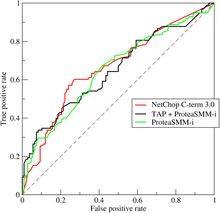
ROC curve of three predictors of peptide cleaving in the proteasome.
A receiver operating characteristic curve, or ROC curve, is a graphical plot that illustrates the diagnostic ability of a binary classifier system as its discrimination threshold is varied. The method was originally developed for operators of military radar receivers starting in 1941, which led to its name.
The ROC curve is created by plotting the true positive rate (TPR) against the false positive rate (FPR) at various threshold settings. The true-positive rate is also known as sensitivity, recall or probability of detection.[10] The false-positive rate is also known as probability of false alarm[10] and can be calculated as (1 − specificity). The ROC can also be thought of as a plot of the power as a function of the Type I Error of the decision rule (when the performance is calculated from just a sample of the population, it can be thought of as estimators of these quantities). The ROC curve is thus the sensitivity or recall as a function of fall-out. In general, if the probability distributions for both detection and false alarm are known, the ROC curve can be generated by plotting the cumulative distribution function (area under the probability distribution from 
ROC analysis provides tools to select possibly optimal models and to discard suboptimal ones independently from (and prior to specifying) the cost context or the class distribution. ROC analysis is related in a direct and natural way to cost/benefit analysis of diagnostic decision making.
The ROC curve was first developed by electrical engineers and radar engineers during World War II for detecting enemy objects in battlefields and was soon introduced to psychology to account for perceptual detection of stimuli. ROC analysis since then has been used in medicine, radiology, biometrics, forecasting of natural hazards,[11] meteorology,[12] model performance assessment,[13] and other areas for many decades and is increasingly used in machine learning and data mining research.
The ROC is also known as a relative operating characteristic curve, because it is a comparison of two operating characteristics (TPR and FPR) as the criterion changes.[14]
Basic concept[edit]
A classification model (classifier or diagnosis[15]) is a mapping of instances between certain classes/groups. Because the classifier or diagnosis result can be an arbitrary real value (continuous output), the classifier boundary between classes must be determined by a threshold value (for instance, to determine whether a person has hypertension based on a blood pressure measure). Or it can be a discrete class label, indicating one of the classes.
Consider a two-class prediction problem (binary classification), in which the outcomes are labeled either as positive (p) or negative (n). There are four possible outcomes from a binary classifier. If the outcome from a prediction is p and the actual value is also p, then it is called a true positive (TP); however if the actual value is n then it is said to be a false positive (FP). Conversely, a true negative (TN) has occurred when both the prediction outcome and the actual value are n, and false negative (FN) is when the prediction outcome is n while the actual value is p.
To get an appropriate example in a real-world problem, consider a diagnostic test that seeks to determine whether a person has a certain disease. A false positive in this case occurs when the person tests positive, but does not actually have the disease. A false negative, on the other hand, occurs when the person tests negative, suggesting they are healthy, when they actually do have the disease.
Let us define an experiment from P positive instances and N negative instances for some condition. The four outcomes can be formulated in a 2×2 contingency table or confusion matrix, as follows:
| Predicted condition | Sources: [16][17][18][19][20][21][22][23][24]
|
||||
| Total population = P + N |
Positive (PP) | Negative (PN) | Informedness, bookmaker informedness (BM) = TPR + TNR − 1 |
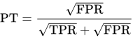
Prevalence threshold (PT) = 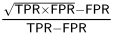
|
|
|
Actual condition |
Positive (P) | True positive (TP), hit |
False negative (FN), type II error, miss, underestimation |
True positive rate (TPR), recall, sensitivity (SEN), probability of detection, hit rate, power = TP/P = 1 − FNR |
False negative rate (FNR), miss rate = FN/P = 1 − TPR |
| Negative (N) | False positive (FP), type I error, false alarm, overestimation |
True negative (TN), correct rejection |
False positive rate (FPR), probability of false alarm, fall-out = FP/N = 1 − TNR |
True negative rate (TNR), specificity (SPC), selectivity = TN/N = 1 − FPR |
|
| Prevalence = P/P + N |
Positive predictive value (PPV), precision = TP/PP = 1 − FDR |
False omission rate (FOR) = FN/PN = 1 − NPV |
Positive likelihood ratio (LR+) = TPR/FPR |
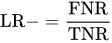
Negative likelihood ratio (LR−) = FNR/TNR |
|
| Accuracy (ACC) = TP + TN/P + N | False discovery rate (FDR) = FP/PP = 1 − PPV |
Negative predictive value (NPV) = TN/PN = 1 − FOR | Markedness (MK), deltaP (Δp) = PPV + NPV − 1 |
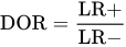
Diagnostic odds ratio (DOR) = LR+/LR− | |
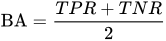
| Balanced accuracy (BA) = TPR + TNR/2 | F1 score = 2 PPV × TPR/PPV + TPR = 2 TP/2 TP + FP + FN |
Fowlkes–Mallows index (FM) = 
|
Matthews correlation coefficient (MCC) =  
|
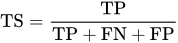
Threat score (TS), critical success index (CSI), Jaccard index = TP/TP + FN + FP |
ROC space[edit]

The ROC space and plots of the four prediction examples.

The ROC space for a «better» and «worse» classifier.
The contingency table can derive several evaluation «metrics» (see infobox). To draw a ROC curve, only the true positive rate (TPR) and false positive rate (FPR) are needed (as functions of some classifier parameter). The TPR defines how many correct positive results occur among all positive samples available during the test. FPR, on the other hand, defines how many incorrect positive results occur among all negative samples available during the test.
A ROC space is defined by FPR and TPR as x and y axes, respectively, which depicts relative trade-offs between true positive (benefits) and false positive (costs). Since TPR is equivalent to sensitivity and FPR is equal to 1 − specificity, the ROC graph is sometimes called the sensitivity vs (1 − specificity) plot. Each prediction result or instance of a confusion matrix represents one point in the ROC space.
The best possible prediction method would yield a point in the upper left corner or coordinate (0,1) of the ROC space, representing 100% sensitivity (no false negatives) and 100% specificity (no false positives). The (0,1) point is also called a perfect classification. A random guess would give a point along a diagonal line (the so-called line of no-discrimination) from the bottom left to the top right corners (regardless of the positive and negative base rates).[25] An intuitive example of random guessing is a decision by flipping coins. As the size of the sample increases, a random classifier’s ROC point tends towards the diagonal line. In the case of a balanced coin, it will tend to the point (0.5, 0.5).
The diagonal divides the ROC space. Points above the diagonal represent good classification results (better than random); points below the line represent bad results (worse than random). Note that the output of a consistently bad predictor could simply be inverted to obtain a good predictor.
Let us look into four prediction results from 100 positive and 100 negative instances:
| A | B | C | C′ | ||||||||||||||||||||||||||||||||||||
|---|---|---|---|---|---|---|---|---|---|---|---|---|---|---|---|---|---|---|---|---|---|---|---|---|---|---|---|---|---|---|---|---|---|---|---|---|---|---|---|
|
|
|
|
||||||||||||||||||||||||||||||||||||
| TPR = 0.63 | TPR = 0.77 | TPR = 0.24 | TPR = 0.76 | ||||||||||||||||||||||||||||||||||||
| FPR = 0.28 | FPR = 0.77 | FPR = 0.88 | FPR = 0.12 | ||||||||||||||||||||||||||||||||||||
| PPV = 0.69 | PPV = 0.50 | PPV = 0.21 | PPV = 0.86 | ||||||||||||||||||||||||||||||||||||
| F1 = 0.66 | F1 = 0.61 | F1 = 0.23 | F1 = 0.81 | ||||||||||||||||||||||||||||||||||||
| ACC = 0.68 | ACC = 0.50 | ACC = 0.18 | ACC = 0.82 |
Plots of the four results above in the ROC space are given in the figure. The result of method A clearly shows the best predictive power among A, B, and C. The result of B lies on the random guess line (the diagonal line), and it can be seen in the table that the accuracy of B is 50%. However, when C is mirrored across the center point (0.5,0.5), the resulting method C′ is even better than A. This mirrored method simply reverses the predictions of whatever method or test produced the C contingency table. Although the original C method has negative predictive power, simply reversing its decisions leads to a new predictive method C′ which has positive predictive power. When the C method predicts p or n, the C′ method would predict n or p, respectively. In this manner, the C′ test would perform the best. The closer a result from a contingency table is to the upper left corner, the better it predicts, but the distance from the random guess line in either direction is the best indicator of how much predictive power a method has. If the result is below the line (i.e. the method is worse than a random guess), all of the method’s predictions must be reversed in order to utilize its power, thereby moving the result above the random guess line.
Curves in ROC space[edit]
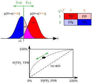
In binary classification, the class prediction for each instance is often made based on a continuous random variable 


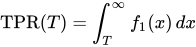
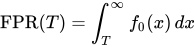
The ROC curve plots parametrically 

For example, imagine that the blood protein levels in diseased people and healthy people are normally distributed with means of 2 g/dL and 1 g/dL respectively. A medical test might measure the level of a certain protein in a blood sample and classify any number above a certain threshold as indicating disease. The experimenter can adjust the threshold (green vertical line in the figure), which will in turn change the false positive rate. Increasing the threshold would result in fewer false positives (and more false negatives), corresponding to a leftward movement on the curve. The actual shape of the curve is determined by how much overlap the two distributions have.
Further interpretations[edit]
Sometimes, the ROC is used to generate a summary statistic. Common versions are:
- the intercept of the ROC curve with the line at 45 degrees orthogonal to the no-discrimination line — the balance point where Sensitivity = 1 — Specificity
- the intercept of the ROC curve with the tangent at 45 degrees parallel to the no-discrimination line that is closest to the error-free point (0,1) — also called Youden’s J statistic and generalized as Informedness[citation needed]
- the area between the ROC curve and the no-discrimination line multiplied by two is called the Gini coefficient. It should not be confused with the measure of statistical dispersion also called Gini coefficient.
- the area between the full ROC curve and the triangular ROC curve including only (0,0), (1,1) and one selected operating point
— Consistency[26]
- the area under the ROC curve, or «AUC» («area under curve»), or A’ (pronounced «a-prime»),[27] or «c-statistic» («concordance statistic»).[28]
- the sensitivity index d′ (pronounced «d-prime»), the distance between the mean of the distribution of activity in the system under noise-alone conditions and its distribution under signal-alone conditions, divided by their standard deviation, under the assumption that both these distributions are normal with the same standard deviation. Under these assumptions, the shape of the ROC is entirely determined by d′.
However, any attempt to summarize the ROC curve into a single number loses information about the pattern of tradeoffs of the particular discriminator algorithm.
Probabilistic interpretation[edit]
When using normalized units, the area under the curve (often referred to as simply the AUC) is equal to the probability that a classifier will rank a randomly chosen positive instance higher than a randomly chosen negative one (assuming ‘positive’ ranks higher than ‘negative’).[29] In other words, when given one randomly selected positive instance and one randomly selected negative instance, AUC is the probability that the classifier will be able to tell which one is which.
This can be seen as follows: the area under the curve is given by (the integral boundaries are reversed as large threshold
a lower value on the x-axis)



where 


Area under the curve[edit]
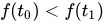
It can be shown that the AUC is closely related to the Mann–Whitney U,[30][31] which tests whether positives are ranked higher than negatives. It is also equivalent to the Wilcoxon test of ranks.[31] For a predictor 
![{displaystyle AUC(f)={frac {sum _{t_{0}in {mathcal {D}}^{0}}sum _{t_{1}in {mathcal {D}}^{1}}{textbf {1}}[f(t_{0})<f(t_{1})]}{|{mathcal {D}}^{0}|cdot |{mathcal {D}}^{1}|}},}](https://wikimedia.org/api/rest_v1/media/math/render/svg/a65ad3f875a1cefbda573962cee7abbb05aa3bcf)
where, ![{textstyle {textbf {1}}[f(t_{0})<f(t_{1})]}](https://wikimedia.org/api/rest_v1/media/math/render/svg/03407a2c3018d99fb12703e2327bfbf84b9ce426)


The AUC is related to the Gini impurity index (

[33]
In this way, it is possible to calculate the AUC by using an average of a number of trapezoidal approximations.
It is also common to calculate the Area Under the ROC Convex Hull (ROC AUCH = ROCH AUC) as any point on the line segment between two prediction results can be achieved by randomly using one or the other system with probabilities proportional to the relative length of the opposite component of the segment.[34] It is also possible to invert concavities – just as in the figure the worse solution can be reflected to become a better solution; concavities can be reflected in any line segment, but this more extreme form of fusion is much more likely to overfit the data.[35]
The machine learning community most often uses the ROC AUC statistic for model comparison.[36] This practice has been questioned because AUC estimates are quite noisy and suffer from other problems.[37][38][39] Nonetheless, the coherence of AUC as a measure of aggregated classification performance has been vindicated, in terms of a uniform rate distribution,[40] and AUC has been linked to a number of other performance metrics such as the Brier score.[41]
Another problem with ROC AUC is that reducing the ROC Curve to a single number ignores the fact that it is about the tradeoffs between the different systems or performance points plotted and not the performance of an individual system, as well as ignoring the possibility of concavity repair, so that related alternative measures such as Informedness[citation needed] or DeltaP are recommended.[26][42] These measures are essentially equivalent to the Gini for a single prediction point with DeltaP’ = Informedness = 2AUC-1, whilst DeltaP = Markedness represents the dual (viz. predicting the prediction from the real class) and their geometric mean is the Matthews correlation coefficient.[citation needed]
Whereas ROC AUC varies between 0 and 1 — with an uninformative classifier yielding 0.5 — the alternative measures known as Informedness,[citation needed] Certainty [26] and Gini Coefficient (in the single parameterization or single system case)[citation needed] all have the advantage that 0 represents chance performance whilst 1 represents perfect performance, and −1 represents the «perverse» case of full informedness always giving the wrong response.[43] Bringing chance performance to 0 allows these alternative scales to be interpreted as Kappa statistics. Informedness has been shown to have desirable characteristics for Machine Learning versus other common definitions of Kappa such as Cohen Kappa and Fleiss Kappa.[citation needed][44]
Sometimes it can be more useful to look at a specific region of the ROC Curve rather than at the whole curve. It is possible to compute partial AUC.[45] For example, one could focus on the region of the curve with low false positive rate, which is often of prime interest for population screening tests.[46] Another common approach for classification problems in which P ≪ N (common in bioinformatics applications) is to use a logarithmic scale for the x-axis.[47]
The ROC area under the curve is also called c-statistic or c statistic.[48]
Other measures[edit]

The Total Operating Characteristic (TOC) also characterizes diagnostic ability while revealing more information than the ROC. For each threshold, ROC reveals two ratios, TP/(TP + FN) and FP/(FP + TN). In other words, ROC reveals 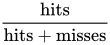


These figures are the TOC and ROC curves using the same data and thresholds.
Consider the point that corresponds to a threshold of 74. The TOC curve shows the number of hits, which is 3, and hence the number of misses, which is 7. Additionally, the TOC curve shows that the number of false alarms is 4 and the number of correct rejections is 16. At any given point in the ROC curve, it is possible to glean values for the ratios of
Detection error tradeoff graph[edit]
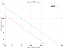
An alternative to the ROC curve is the detection error tradeoff (DET) graph, which plots the false negative rate (missed detections) vs. the false positive rate (false alarms) on non-linearly transformed x- and y-axes. The transformation function is the quantile function of the normal distribution, i.e., the inverse of the cumulative normal distribution. It is, in fact, the same transformation as zROC, below, except that the complement of the hit rate, the miss rate or false negative rate, is used. This alternative spends more graph area on the region of interest. Most of the ROC area is of little interest; one primarily cares about the region tight against the y-axis and the top left corner – which, because of using miss rate instead of its complement, the hit rate, is the lower left corner in a DET plot. Furthermore, DET graphs have the useful property of linearity and a linear threshold behavior for normal distributions.[51] The DET plot is used extensively in the automatic speaker recognition community, where the name DET was first used. The analysis of the ROC performance in graphs with this warping of the axes was used by psychologists in perception studies halfway through the 20th century,[citation needed] where this was dubbed «double probability paper».[52]
Z-score[edit]
If a standard score is applied to the ROC curve, the curve will be transformed into a straight line.[53] This z-score is based on a normal distribution with a mean of zero and a standard deviation of one. In memory strength theory, one must assume that the zROC is not only linear, but has a slope of 1.0. The normal distributions of targets (studied objects that the subjects need to recall) and lures (non studied objects that the subjects attempt to recall) is the factor causing the zROC to be linear.
The linearity of the zROC curve depends on the standard deviations of the target and lure strength distributions. If the standard deviations are equal, the slope will be 1.0. If the standard deviation of the target strength distribution is larger than the standard deviation of the lure strength distribution, then the slope will be smaller than 1.0. In most studies, it has been found that the zROC curve slopes constantly fall below 1, usually between 0.5 and 0.9.[54] Many experiments yielded a zROC slope of 0.8. A slope of 0.8 implies that the variability of the target strength distribution is 25% larger than the variability of the lure strength distribution.[55]
Another variable used is d’ (d prime) (discussed above in «Other measures»), which can easily be expressed in terms of z-values. Although d‘ is a commonly used parameter, it must be recognized that it is only relevant when strictly adhering to the very strong assumptions of strength theory made above.[56]
The z-score of an ROC curve is always linear, as assumed, except in special situations. The Yonelinas familiarity-recollection model is a two-dimensional account of recognition memory. Instead of the subject simply answering yes or no to a specific input, the subject gives the input a feeling of familiarity, which operates like the original ROC curve. What changes, though, is a parameter for Recollection (R). Recollection is assumed to be all-or-none, and it trumps familiarity. If there were no recollection component, zROC would have a predicted slope of 1. However, when adding the recollection component, the zROC curve will be concave up, with a decreased slope. This difference in shape and slope result from an added element of variability due to some items being recollected. Patients with anterograde amnesia are unable to recollect, so their Yonelinas zROC curve would have a slope close to 1.0.[57]
History[edit]
The ROC curve was first used during World War II for the analysis of radar signals before it was employed in signal detection theory.[58] Following the attack on Pearl Harbor in 1941, the United States army began new research to increase the prediction of correctly detected Japanese aircraft from their radar signals. For these purposes they measured the ability of a radar receiver operator to make these important distinctions, which was called the Receiver Operating Characteristic.[59]
In the 1950s, ROC curves were employed in psychophysics to assess human (and occasionally non-human animal) detection of weak signals.[58] In medicine, ROC analysis has been extensively used in the evaluation of diagnostic tests.[60][61] ROC curves are also used extensively in epidemiology and medical research and are frequently mentioned in conjunction with evidence-based medicine. In radiology, ROC analysis is a common technique to evaluate new radiology techniques.[62] In the social sciences, ROC analysis is often called the ROC Accuracy Ratio, a common technique for judging the accuracy of default probability models.
ROC curves are widely used in laboratory medicine to assess the diagnostic accuracy of a test, to choose the optimal cut-off of a test and to compare diagnostic accuracy of several tests.
ROC curves also proved useful for the evaluation of machine learning techniques. The first application of ROC in machine learning was by Spackman who demonstrated the value of ROC curves in comparing and evaluating different classification algorithms.[63]
ROC curves are also used in verification of forecasts in meteorology.[64]
ROC curves beyond binary classification[edit]
The extension of ROC curves for classification problems with more than two classes is cumbersome. Two common approaches for when there are multiple classes are (1) average over all pairwise AUC values[65] and (2) compute the volume under surface (VUS).[66][67] To average over all pairwise classes, one computes the AUC for each pair of classes, using only the examples from those two classes as if there were no other classes, and then averages these AUC values over all possible pairs. When there are c classes there will be c(c − 1) / 2 possible pairs of classes.
The volume under surface approach has one plot a hypersurface rather than a curve and then measure the hypervolume under that hypersurface. Every possible decision rule that one might use for a classifier for c classes can be described in terms of its true positive rates (TPR1, …, TPRc). It is this set of rates that defines a point, and the set of all possible decision rules yields a cloud of points that define the hypersurface. With this definition, the VUS is the probability that the classifier will be able to correctly label all c examples when it is given a set that has one randomly selected example from each class. The implementation of a classifier that knows that its input set consists of one example from each class might first compute a goodness-of-fit score for each of the c2 possible pairings of an example to a class, and then employ the Hungarian algorithm to maximize the sum of the c selected scores over all c! possible ways to assign exactly one example to each class.
Given the success of ROC curves for the assessment of classification models, the extension of ROC curves for other supervised tasks has also been investigated. Notable proposals for regression problems are the so-called regression error characteristic (REC) Curves [68] and the Regression ROC (RROC) curves.[69] In the latter, RROC curves become extremely similar to ROC curves for classification, with the notions of asymmetry, dominance and convex hull. Also, the area under RROC curves is proportional to the error variance of the regression model.
See also[edit]
- Brier score
- Coefficient of determination
- Constant false alarm rate
- Detection error tradeoff
- Detection theory
- F1 score
- False alarm
- Hypothesis tests for accuracy
- Precision and recall
- ROCCET
- Sensitivity and specificity
- Total operating characteristic
References[edit]
- ^ Fawcett, Tom (2006). «An Introduction to ROC Analysis» (PDF). Pattern Recognition Letters. 27 (8): 861–874. doi:10.1016/j.patrec.2005.10.010.
- ^ Piryonesi S. Madeh; El-Diraby Tamer E. (2020-03-01). «Data Analytics in Asset Management: Cost-Effective Prediction of the Pavement Condition Index». Journal of Infrastructure Systems. 26 (1): 04019036. doi:10.1061/(ASCE)IS.1943-555X.0000512.
- ^ Powers, David M. W. (2011). «Evaluation: From Precision, Recall and F-Measure to ROC, Informedness, Markedness & Correlation». Journal of Machine Learning Technologies. 2 (1): 37–63.
- ^ Ting, Kai Ming (2011). Sammut, Claude; Webb, Geoffrey I. (eds.). Encyclopedia of machine learning. Springer. doi:10.1007/978-0-387-30164-8. ISBN 978-0-387-30164-8.
- ^ Brooks, Harold; Brown, Barb; Ebert, Beth; Ferro, Chris; Jolliffe, Ian; Koh, Tieh-Yong; Roebber, Paul; Stephenson, David (2015-01-26). «WWRP/WGNE Joint Working Group on Forecast Verification Research». Collaboration for Australian Weather and Climate Research. World Meteorological Organisation. Retrieved 2019-07-17.
- ^ Chicco D.; Jurman G. (January 2020). «The advantages of the Matthews correlation coefficient (MCC) over F1 score and accuracy in binary classification evaluation». BMC Genomics. 21 (1): 6-1–6-13. doi:10.1186/s12864-019-6413-7. PMC 6941312. PMID 31898477.
- ^ Chicco D.; Toetsch N.; Jurman G. (February 2021). «The Matthews correlation coefficient (MCC) is more reliable than balanced accuracy, bookmaker informedness, and markedness in two-class confusion matrix evaluation». BioData Mining. 14 (13): 1-22. doi:10.1186/s13040-021-00244-z. PMC 7863449. PMID 33541410.
- ^ Tharwat A. (August 2018). «Classification assessment methods». Applied Computing and Informatics. doi:10.1016/j.aci.2018.08.003.
- ^ Balayla, Jacques (2020). «Prevalence threshold (ϕe) and the geometry of screening curves». PLoS One. 15 (10). doi:10.1371/journal.pone.0240215.
- ^ a b «Detector Performance Analysis Using ROC Curves — MATLAB & Simulink Example». www.mathworks.com. Retrieved 11 August 2016.
- ^ Peres, D. J.; Cancelliere, A. (2014-12-08). «Derivation and evaluation of landslide-triggering thresholds by a Monte Carlo approach». Hydrol. Earth Syst. Sci. 18 (12): 4913–4931. Bibcode:2014HESS…18.4913P. doi:10.5194/hess-18-4913-2014. ISSN 1607-7938.
- ^ Murphy, Allan H. (1996-03-01). «The Finley Affair: A Signal Event in the History of Forecast Verification». Weather and Forecasting. 11 (1): 3–20. Bibcode:1996WtFor..11….3M. doi:10.1175/1520-0434(1996)011<0003:tfaase>2.0.co;2. ISSN 0882-8156.
- ^ Peres, D. J.; Iuppa, C.; Cavallaro, L.; Cancelliere, A.; Foti, E. (2015-10-01). «Significant wave height record extension by neural networks and reanalysis wind data». Ocean Modelling. 94: 128–140. Bibcode:2015OcMod..94..128P. doi:10.1016/j.ocemod.2015.08.002.
- ^ Swets, John A.; Signal detection theory and ROC analysis in psychology and diagnostics : collected papers, Lawrence Erlbaum Associates, Mahwah, NJ, 1996
- ^ Sushkova, Olga; Morozov, Alexei; Gabova, Alexandra; Karabanov, Alexei; Illarioshkin, Sergey (2021). «A Statistical Method for Exploratory Data Analysis Based on 2D and 3D Area under Curve Diagrams: Parkinson’s Disease Investigation». Sensors. 21 (14): 4700. doi:10.3390/s21144700. PMC 8309570. PMID 34300440.
- ^
Balayla, Jacques (2020). «Prevalence threshold (ϕe) and the geometry of screening curves». PLoS One. 15 (10). doi:10.1371/journal.pone.0240215. - ^
Fawcett, Tom (2006). «An Introduction to ROC Analysis» (PDF). Pattern Recognition Letters. 27 (8): 861–874. doi:10.1016/j.patrec.2005.10.010. - ^
Piryonesi S. Madeh; El-Diraby Tamer E. (2020-03-01). «Data Analytics in Asset Management: Cost-Effective Prediction of the Pavement Condition Index». Journal of Infrastructure Systems. 26 (1): 04019036. doi:10.1061/(ASCE)IS.1943-555X.0000512. - ^
Powers, David M. W. (2011). «Evaluation: From Precision, Recall and F-Measure to ROC, Informedness, Markedness & Correlation». Journal of Machine Learning Technologies. 2 (1): 37–63. - ^
Ting, Kai Ming (2011). Sammut, Claude; Webb, Geoffrey I. (eds.). Encyclopedia of machine learning. Springer. doi:10.1007/978-0-387-30164-8. ISBN 978-0-387-30164-8. - ^
Brooks, Harold; Brown, Barb; Ebert, Beth; Ferro, Chris; Jolliffe, Ian; Koh, Tieh-Yong; Roebber, Paul; Stephenson, David (2015-01-26). «WWRP/WGNE Joint Working Group on Forecast Verification Research». Collaboration for Australian Weather and Climate Research. World Meteorological Organisation. Retrieved 2019-07-17. - ^
Chicco D, Jurman G (January 2020). «The advantages of the Matthews correlation coefficient (MCC) over F1 score and accuracy in binary classification evaluation». BMC Genomics. 21 (1): 6-1–6-13. doi:10.1186/s12864-019-6413-7. PMC 6941312. PMID 31898477. - ^
Chicco D, Toetsch N, Jurman G (February 2021). «The Matthews correlation coefficient (MCC) is more reliable than balanced accuracy, bookmaker informedness, and markedness in two-class confusion matrix evaluation». BioData Mining. 14 (13): 1-22. doi:10.1186/s13040-021-00244-z. PMC 7863449. PMID 33541410. - ^
Tharwat A. (August 2018). «Classification assessment methods». Applied Computing and Informatics. doi:10.1016/j.aci.2018.08.003. - ^ «classification — AUC-ROC of a random classifier». Data Science Stack Exchange. Retrieved 2020-11-30.
- ^ a b c Powers, David MW (2012). «ROC-ConCert: ROC-Based Measurement of Consistency and Certainty» (PDF). Spring Congress on Engineering and Technology (SCET). Vol. 2. IEEE. pp. 238–241.[dead link]
- ^ Fogarty, James; Baker, Ryan S.; Hudson, Scott E. (2005). «Case studies in the use of ROC curve analysis for sensor-based estimates in human computer interaction». ACM International Conference Proceeding Series, Proceedings of Graphics Interface 2005. Waterloo, ON: Canadian Human-Computer Communications Society.
- ^ Hastie, Trevor; Tibshirani, Robert; Friedman, Jerome H. (2009). The elements of statistical learning: data mining, inference, and prediction (2nd ed.).
- ^ Fawcett, Tom (2006); An introduction to ROC analysis, Pattern Recognition Letters, 27, 861–874.
- ^ Hanley, James A.; McNeil, Barbara J. (1982). «The Meaning and Use of the Area under a Receiver Operating Characteristic (ROC) Curve». Radiology. 143 (1): 29–36. doi:10.1148/radiology.143.1.7063747. PMID 7063747. S2CID 10511727.
- ^ a b Mason, Simon J.; Graham, Nicholas E. (2002). «Areas beneath the relative operating characteristics (ROC) and relative operating levels (ROL) curves: Statistical significance and interpretation» (PDF). Quarterly Journal of the Royal Meteorological Society. 128 (584): 2145–2166. Bibcode:2002QJRMS.128.2145M. CiteSeerX 10.1.1.458.8392. doi:10.1256/003590002320603584. Archived from the original (PDF) on 2008-11-20.
- ^ Calders, Toon; Jaroszewicz, Szymon (2007). Kok, Joost N.; Koronacki, Jacek; Lopez de Mantaras, Ramon; Matwin, Stan; Mladenič, Dunja; Skowron, Andrzej (eds.). «Efficient AUC Optimization for Classification». Knowledge Discovery in Databases: PKDD 2007. Lecture Notes in Computer Science. Berlin, Heidelberg: Springer. 4702: 42–53. doi:10.1007/978-3-540-74976-9_8. ISBN 978-3-540-74976-9.
- ^ Hand, David J.; and Till, Robert J. (2001); A simple generalization of the area under the ROC curve for multiple class classification problems, Machine Learning, 45, 171–186.
- ^ Provost, F.; Fawcett, T. (2001). «Robust classification for imprecise environments». Machine Learning. 42 (3): 203–231. arXiv:cs/0009007. doi:10.1023/a:1007601015854. S2CID 5415722.
- ^ Flach, P.A.; Wu, S. (2005). «Repairing concavities in ROC curves.» (PDF). 19th International Joint Conference on Artificial Intelligence (IJCAI’05). pp. 702–707.
- ^ Hanley, James A.; McNeil, Barbara J. (1983-09-01). «A method of comparing the areas under receiver operating characteristic curves derived from the same cases». Radiology. 148 (3): 839–843. doi:10.1148/radiology.148.3.6878708. PMID 6878708.
- ^ Hanczar, Blaise; Hua, Jianping; Sima, Chao; Weinstein, John; Bittner, Michael; Dougherty, Edward R (2010). «Small-sample precision of ROC-related estimates». Bioinformatics. 26 (6): 822–830. doi:10.1093/bioinformatics/btq037. PMID 20130029.
- ^ Lobo, Jorge M.; Jiménez-Valverde, Alberto; Real, Raimundo (2008). «AUC: a misleading measure of the performance of predictive distribution models». Global Ecology and Biogeography. 17 (2): 145–151. doi:10.1111/j.1466-8238.2007.00358.x. S2CID 15206363.
- ^ Hand, David J (2009). «Measuring classifier performance: A coherent alternative to the area under the ROC curve». Machine Learning. 77: 103–123. doi:10.1007/s10994-009-5119-5.
- ^ Flach, P.A.; Hernandez-Orallo, J.; Ferri, C. (2011). «A coherent interpretation of AUC as a measure of aggregated classification performance.» (PDF). Proceedings of the 28th International Conference on Machine Learning (ICML-11). pp. 657–664.
- ^ Hernandez-Orallo, J.; Flach, P.A.; Ferri, C. (2012). «A unified view of performance metrics: translating threshold choice into expected classification loss» (PDF). Journal of Machine Learning Research. 13: 2813–2869.
- ^ Powers, David M.W. (2012). «The Problem of Area Under the Curve». International Conference on Information Science and Technology.
- ^ Powers, David M. W. (2003). «Recall and Precision versus the Bookmaker» (PDF). Proceedings of the International Conference on Cognitive Science (ICSC-2003), Sydney Australia, 2003, pp. 529–534.
- ^ Powers, David M. W. (2012). «The Problem with Kappa» (PDF). Conference of the European Chapter of the Association for Computational Linguistics (EACL2012) Joint ROBUS-UNSUP Workshop. Archived from the original (PDF) on 2016-05-18. Retrieved 2012-07-20.
- ^ McClish, Donna Katzman (1989-08-01). «Analyzing a Portion of the ROC Curve». Medical Decision Making. 9 (3): 190–195. doi:10.1177/0272989X8900900307. PMID 2668680. S2CID 24442201.
- ^ Dodd, Lori E.; Pepe, Margaret S. (2003). «Partial AUC Estimation and Regression». Biometrics. 59 (3): 614–623. doi:10.1111/1541-0420.00071. PMID 14601762.
- ^ Karplus, Kevin (2011); Better than Chance: the importance of null models, University of California, Santa Cruz, in Proceedings of the First International Workshop on Pattern Recognition in Proteomics, Structural Biology and Bioinformatics (PR PS BB 2011)
- ^ «C-Statistic: Definition, Examples, Weighting and Significance». Statistics How To. August 28, 2016.
- ^ Pontius, Robert Gilmore; Parmentier, Benoit (2014). «Recommendations for using the Relative Operating Characteristic (ROC)». Landscape Ecology. 29 (3): 367–382. doi:10.1007/s10980-013-9984-8. S2CID 15924380.
- ^ Pontius, Robert Gilmore; Si, Kangping (2014). «The total operating characteristic to measure diagnostic ability for multiple thresholds». International Journal of Geographical Information Science. 28 (3): 570–583. doi:10.1080/13658816.2013.862623. S2CID 29204880.
- ^ Navratil, J.; Klusacek, D. (2007-04-01). On Linear DETs. 2007 IEEE International Conference on Acoustics, Speech and Signal Processing — ICASSP ’07. Vol. 4. pp. IV–229–IV–232. doi:10.1109/ICASSP.2007.367205. ISBN 978-1-4244-0727-9. S2CID 18173315.
- ^ Dev P. Chakraborty (December 14, 2017). «double+probability+paper»&pg=PT214 Observer Performance Methods for Diagnostic Imaging: Foundations, Modeling, and Applications with R-Based Examples. CRC Press. p. 214. ISBN 9781351230711. Retrieved July 11, 2019.
- ^ MacMillan, Neil A.; Creelman, C. Douglas (2005). Detection Theory: A User’s Guide (2nd ed.). Mahwah, NJ: Lawrence Erlbaum Associates. ISBN 978-1-4106-1114-7.
- ^ Glanzer, Murray; Kisok, Kim; Hilford, Andy; Adams, John K. (1999). «Slope of the receiver-operating characteristic in recognition memory». Journal of Experimental Psychology: Learning, Memory, and Cognition. 25 (2): 500–513. doi:10.1037/0278-7393.25.2.500.
- ^ Ratcliff, Roger; McCoon, Gail; Tindall, Michael (1994). «Empirical generality of data from recognition memory ROC functions and implications for GMMs». Journal of Experimental Psychology: Learning, Memory, and Cognition. 20 (4): 763–785. CiteSeerX 10.1.1.410.2114. doi:10.1037/0278-7393.20.4.763.
- ^ Zhang, Jun; Mueller, Shane T. (2005). «A note on ROC analysis and non-parametric estimate of sensitivity». Psychometrika. 70: 203–212. CiteSeerX 10.1.1.162.1515. doi:10.1007/s11336-003-1119-8. S2CID 122355230.
- ^ Yonelinas, Andrew P.; Kroll, Neal E. A.; Dobbins, Ian G.; Lazzara, Michele; Knight, Robert T. (1998). «Recollection and familiarity deficits in amnesia: Convergence of remember-know, process dissociation, and receiver operating characteristic data». Neuropsychology. 12 (3): 323–339. doi:10.1037/0894-4105.12.3.323. PMID 9673991.
- ^ a b Green, David M.; Swets, John A. (1966). Signal detection theory and psychophysics. New York, NY: John Wiley and Sons Inc. ISBN 978-0-471-32420-1.
- ^ «Using the Receiver Operating Characteristic (ROC) curve to analyze a classification model: A final note of historical interest» (PDF). Department of Mathematics, University of Utah. Department of Mathematics, University of Utah. Archived (PDF) from the original on 2020-08-22. Retrieved May 25, 2017.
- ^ Zweig, Mark H.; Campbell, Gregory (1993). «Receiver-operating characteristic (ROC) plots: a fundamental evaluation tool in clinical medicine» (PDF). Clinical Chemistry. 39 (8): 561–577. doi:10.1093/clinchem/39.4.561. PMID 8472349.
- ^ Pepe, Margaret S. (2003). The statistical evaluation of medical tests for classification and prediction. New York, NY: Oxford. ISBN 978-0-19-856582-6.
- ^ Obuchowski, Nancy A. (2003). «Receiver operating characteristic curves and their use in radiology». Radiology. 229 (1): 3–8. doi:10.1148/radiol.2291010898. PMID 14519861.
- ^ Spackman, Kent A. (1989). «Signal detection theory: Valuable tools for evaluating inductive learning». Proceedings of the Sixth International Workshop on Machine Learning. San Mateo, CA: Morgan Kaufmann. pp. 160–163.
- ^ Kharin, Viatcheslav (2003). «On the ROC score of probability forecasts». Journal of Climate. 16 (24): 4145–4150. Bibcode:2003JCli…16.4145K. doi:10.1175/1520-0442(2003)016<4145:OTRSOP>2.0.CO;2.
- ^ Till, D.J.; Hand, R.J. (2001). «A Simple Generalisation of the Area Under the ROC Curve for Multiple Class Classification Problems». Machine Learning. 45 (2): 171–186. doi:10.1023/A:1010920819831.
- ^ Mossman, D. (1999). «Three-way ROCs». Medical Decision Making. 19 (1): 78–89. doi:10.1177/0272989×9901900110. PMID 9917023. S2CID 24623127.
- ^ Ferri, C.; Hernandez-Orallo, J.; Salido, M.A. (2003). «Volume under the ROC Surface for Multi-class Problems». Machine Learning: ECML 2003. pp. 108–120.
- ^ Bi, J.; Bennett, K.P. (2003). «Regression error characteristic curves» (PDF). Twentieth International Conference on Machine Learning (ICML-2003). Washington, DC.
- ^ Hernandez-Orallo, J. (2013). «ROC curves for regression». Pattern Recognition. 46 (12): 3395–3411. doi:10.1016/j.patcog.2013.06.014. hdl:10251/40252.
External links[edit]
- ROC demo
- another ROC demo
- ROC video explanation
- An Introduction to the Total Operating Characteristic: Utility in Land Change Model Evaluation
- How to run the TOC Package in R
- TOC R package on Github
- Excel Workbook for generating TOC curves
Further reading[edit]
- Balakrishnan, Narayanaswamy (1991); Handbook of the Logistic Distribution, Marcel Dekker, Inc., ISBN 978-0-8247-8587-1
- Brown, Christopher D.; Davis, Herbert T. (2006). «Receiver operating characteristic curves and related decision measures: a tutorial». Chemometrics and Intelligent Laboratory Systems. 80: 24–38. doi:10.1016/j.chemolab.2005.05.004.
- Rotello, Caren M.; Heit, Evan; Dubé, Chad (2014). «When more data steer us wrong: replications with the wrong dependent measure perpetuate erroneous conclusions» (PDF). Psychonomic Bulletin & Review. 22 (4): 944–954. doi:10.3758/s13423-014-0759-2. PMID 25384892. S2CID 6046065.
- Fawcett, Tom (2004). «ROC Graphs: Notes and Practical Considerations for Researchers» (PDF). Pattern Recognition Letters. 27 (8): 882–891. CiteSeerX 10.1.1.145.4649. doi:10.1016/j.patrec.2005.10.012.
- Gonen, Mithat (2007); Analyzing Receiver Operating Characteristic Curves Using SAS, SAS Press, ISBN 978-1-59994-298-8
- Green, William H., (2003) Econometric Analysis, fifth edition, Prentice Hall, ISBN 0-13-066189-9
- Heagerty, Patrick J.; Lumley, Thomas; Pepe, Margaret S. (2000). «Time-dependent ROC Curves for Censored Survival Data and a Diagnostic Marker». Biometrics. 56 (2): 337–344. doi:10.1111/j.0006-341x.2000.00337.x. PMID 10877287. S2CID 8822160.
- Hosmer, David W.; and Lemeshow, Stanley (2000); Applied Logistic Regression, 2nd ed., New York, NY: Wiley, ISBN 0-471-35632-8
- Lasko, Thomas A.; Bhagwat, Jui G.; Zou, Kelly H.; Ohno-Machado, Lucila (2005). «The use of receiver operating characteristic curves in biomedical informatics». Journal of Biomedical Informatics. 38 (5): 404–415. CiteSeerX 10.1.1.97.9674. doi:10.1016/j.jbi.2005.02.008. PMID 16198999.
- Mas, Jean-François; Filho, Britaldo Soares; Pontius, Jr, Robert Gilmore; Gutiérrez, Michelle Farfán; Rodrigues, Hermann (2013). «A suite of tools for ROC analysis of spatial models». ISPRS International Journal of Geo-Information. 2 (3): 869–887. Bibcode:2013IJGI….2..869M. doi:10.3390/ijgi2030869.
- Pontius, Jr, Robert Gilmore; Parmentier, Benoit (2014). «Recommendations for using the Relative Operating Characteristic (ROC)». Landscape Ecology. 29 (3): 367–382. doi:10.1007/s10980-013-9984-8. S2CID 15924380.
- Pontius, Jr, Robert Gilmore; Pacheco, Pablo (2004). «Calibration and validation of a model of forest disturbance in the Western Ghats, India 1920–1990». GeoJournal. 61 (4): 325–334. doi:10.1007/s10708-004-5049-5. S2CID 155073463.
- Pontius, Jr, Robert Gilmore; Batchu, Kiran (2003). «Using the relative operating characteristic to quantify certainty in prediction of location of land cover change in India». Transactions in GIS. 7 (4): 467–484. doi:10.1111/1467-9671.00159. S2CID 14452746.
- Pontius, Jr, Robert Gilmore; Schneider, Laura (2001). «Land-use change model validation by a ROC method for the Ipswich watershed, Massachusetts, USA». Agriculture, Ecosystems & Environment. 85 (1–3): 239–248. doi:10.1016/S0167-8809(01)00187-6.
- Stephan, Carsten; Wesseling, Sebastian; Schink, Tania; Jung, Klaus (2003). «Comparison of Eight Computer Programs for Receiver-Operating Characteristic Analysis». Clinical Chemistry. 49 (3): 433–439. doi:10.1373/49.3.433. PMID 12600955.
- Swets, John A.; Dawes, Robyn M.; and Monahan, John (2000); Better Decisions through Science, Scientific American, October, pp. 82–87
- Zou, Kelly H.; O’Malley, A. James; Mauri, Laura (2007). «Receiver-operating characteristic analysis for evaluating diagnostic tests and predictive models». Circulation. 115 (5): 654–7. doi:10.1161/circulationaha.105.594929. PMID 17283280.
- Zhou, Xiao-Hua; Obuchowski, Nancy A.; McClish, Donna K. (2002). Statistical Methods in Diagnostic Medicine. New York, NY: Wiley & Sons. ISBN 978-0-471-34772-9.
Sources: Fawcett (2006),[1] Piryonesi and El-Diraby (2020),[2] |
ROC curve of three predictors of peptide cleaving in the proteasome.
A receiver operating characteristic curve, or ROC curve, is a graphical plot that illustrates the diagnostic ability of a binary classifier system as its discrimination threshold is varied. The method was originally developed for operators of military radar receivers starting in 1941, which led to its name.
The ROC curve is created by plotting the true positive rate (TPR) against the false positive rate (FPR) at various threshold settings. The true-positive rate is also known as sensitivity, recall or probability of detection.[10] The false-positive rate is also known as probability of false alarm[10] and can be calculated as (1 − specificity). The ROC can also be thought of as a plot of the power as a function of the Type I Error of the decision rule (when the performance is calculated from just a sample of the population, it can be thought of as estimators of these quantities). The ROC curve is thus the sensitivity or recall as a function of fall-out. In general, if the probability distributions for both detection and false alarm are known, the ROC curve can be generated by plotting the cumulative distribution function (area under the probability distribution from
ROC analysis provides tools to select possibly optimal models and to discard suboptimal ones independently from (and prior to specifying) the cost context or the class distribution. ROC analysis is related in a direct and natural way to cost/benefit analysis of diagnostic decision making.
The ROC curve was first developed by electrical engineers and radar engineers during World War II for detecting enemy objects in battlefields and was soon introduced to psychology to account for perceptual detection of stimuli. ROC analysis since then has been used in medicine, radiology, biometrics, forecasting of natural hazards,[11] meteorology,[12] model performance assessment,[13] and other areas for many decades and is increasingly used in machine learning and data mining research.
The ROC is also known as a relative operating characteristic curve, because it is a comparison of two operating characteristics (TPR and FPR) as the criterion changes.[14]
Basic concept[edit]
A classification model (classifier or diagnosis[15]) is a mapping of instances between certain classes/groups. Because the classifier or diagnosis result can be an arbitrary real value (continuous output), the classifier boundary between classes must be determined by a threshold value (for instance, to determine whether a person has hypertension based on a blood pressure measure). Or it can be a discrete class label, indicating one of the classes.
Consider a two-class prediction problem (binary classification), in which the outcomes are labeled either as positive (p) or negative (n). There are four possible outcomes from a binary classifier. If the outcome from a prediction is p and the actual value is also p, then it is called a true positive (TP); however if the actual value is n then it is said to be a false positive (FP). Conversely, a true negative (TN) has occurred when both the prediction outcome and the actual value are n, and false negative (FN) is when the prediction outcome is n while the actual value is p.
To get an appropriate example in a real-world problem, consider a diagnostic test that seeks to determine whether a person has a certain disease. A false positive in this case occurs when the person tests positive, but does not actually have the disease. A false negative, on the other hand, occurs when the person tests negative, suggesting they are healthy, when they actually do have the disease.
Let us define an experiment from P positive instances and N negative instances for some condition. The four outcomes can be formulated in a 2×2 contingency table or confusion matrix, as follows:
| Predicted condition | Sources: [16][17][18][19][20][21][22][23][24]
|
||||
| Total population = P + N |
Positive (PP) | Negative (PN) | Informedness, bookmaker informedness (BM) = TPR + TNR − 1 |
Prevalence threshold (PT) =
|
|
|
Actual condition |
Positive (P) | True positive (TP), hit |
False negative (FN), type II error, miss, underestimation |
True positive rate (TPR), recall, sensitivity (SEN), probability of detection, hit rate, power = TP/P = 1 − FNR |
False negative rate (FNR), miss rate = FN/P = 1 − TPR |
| Negative (N) | False positive (FP), type I error, false alarm, overestimation |
True negative (TN), correct rejection |
False positive rate (FPR), probability of false alarm, fall-out = FP/N = 1 − TNR |
True negative rate (TNR), specificity (SPC), selectivity = TN/N = 1 − FPR |
|
| Prevalence = P/P + N |
Positive predictive value (PPV), precision = TP/PP = 1 − FDR |
False omission rate (FOR) = FN/PN = 1 − NPV |
Positive likelihood ratio (LR+) = TPR/FPR |
Negative likelihood ratio (LR−) = FNR/TNR |
|
| Accuracy (ACC) = TP + TN/P + N | False discovery rate (FDR) = FP/PP = 1 − PPV |
Negative predictive value (NPV) = TN/PN = 1 − FOR | Markedness (MK), deltaP (Δp) = PPV + NPV − 1 |
Diagnostic odds ratio (DOR) = LR+/LR− | |
| Balanced accuracy (BA) = TPR + TNR/2 | F1 score = 2 PPV × TPR/PPV + TPR = 2 TP/2 TP + FP + FN |
Fowlkes–Mallows index (FM) =
|
Matthews correlation coefficient (MCC) =
|
Threat score (TS), critical success index (CSI), Jaccard index = TP/TP + FN + FP |
ROC space[edit]
The ROC space and plots of the four prediction examples.
The ROC space for a «better» and «worse» classifier.
The contingency table can derive several evaluation «metrics» (see infobox). To draw a ROC curve, only the true positive rate (TPR) and false positive rate (FPR) are needed (as functions of some classifier parameter). The TPR defines how many correct positive results occur among all positive samples available during the test. FPR, on the other hand, defines how many incorrect positive results occur among all negative samples available during the test.
A ROC space is defined by FPR and TPR as x and y axes, respectively, which depicts relative trade-offs between true positive (benefits) and false positive (costs). Since TPR is equivalent to sensitivity and FPR is equal to 1 − specificity, the ROC graph is sometimes called the sensitivity vs (1 − specificity) plot. Each prediction result or instance of a confusion matrix represents one point in the ROC space.
The best possible prediction method would yield a point in the upper left corner or coordinate (0,1) of the ROC space, representing 100% sensitivity (no false negatives) and 100% specificity (no false positives). The (0,1) point is also called a perfect classification. A random guess would give a point along a diagonal line (the so-called line of no-discrimination) from the bottom left to the top right corners (regardless of the positive and negative base rates).[25] An intuitive example of random guessing is a decision by flipping coins. As the size of the sample increases, a random classifier’s ROC point tends towards the diagonal line. In the case of a balanced coin, it will tend to the point (0.5, 0.5).
The diagonal divides the ROC space. Points above the diagonal represent good classification results (better than random); points below the line represent bad results (worse than random). Note that the output of a consistently bad predictor could simply be inverted to obtain a good predictor.
Let us look into four prediction results from 100 positive and 100 negative instances:
| A | B | C | C′ | ||||||||||||||||||||||||||||||||||||
|---|---|---|---|---|---|---|---|---|---|---|---|---|---|---|---|---|---|---|---|---|---|---|---|---|---|---|---|---|---|---|---|---|---|---|---|---|---|---|---|
|
|
|
|
||||||||||||||||||||||||||||||||||||
| TPR = 0.63 | TPR = 0.77 | TPR = 0.24 | TPR = 0.76 | ||||||||||||||||||||||||||||||||||||
| FPR = 0.28 | FPR = 0.77 | FPR = 0.88 | FPR = 0.12 | ||||||||||||||||||||||||||||||||||||
| PPV = 0.69 | PPV = 0.50 | PPV = 0.21 | PPV = 0.86 | ||||||||||||||||||||||||||||||||||||
| F1 = 0.66 | F1 = 0.61 | F1 = 0.23 | F1 = 0.81 | ||||||||||||||||||||||||||||||||||||
| ACC = 0.68 | ACC = 0.50 | ACC = 0.18 | ACC = 0.82 |
Plots of the four results above in the ROC space are given in the figure. The result of method A clearly shows the best predictive power among A, B, and C. The result of B lies on the random guess line (the diagonal line), and it can be seen in the table that the accuracy of B is 50%. However, when C is mirrored across the center point (0.5,0.5), the resulting method C′ is even better than A. This mirrored method simply reverses the predictions of whatever method or test produced the C contingency table. Although the original C method has negative predictive power, simply reversing its decisions leads to a new predictive method C′ which has positive predictive power. When the C method predicts p or n, the C′ method would predict n or p, respectively. In this manner, the C′ test would perform the best. The closer a result from a contingency table is to the upper left corner, the better it predicts, but the distance from the random guess line in either direction is the best indicator of how much predictive power a method has. If the result is below the line (i.e. the method is worse than a random guess), all of the method’s predictions must be reversed in order to utilize its power, thereby moving the result above the random guess line.
Curves in ROC space[edit]
In binary classification, the class prediction for each instance is often made based on a continuous random variable
The ROC curve plots parametrically
For example, imagine that the blood protein levels in diseased people and healthy people are normally distributed with means of 2 g/dL and 1 g/dL respectively. A medical test might measure the level of a certain protein in a blood sample and classify any number above a certain threshold as indicating disease. The experimenter can adjust the threshold (green vertical line in the figure), which will in turn change the false positive rate. Increasing the threshold would result in fewer false positives (and more false negatives), corresponding to a leftward movement on the curve. The actual shape of the curve is determined by how much overlap the two distributions have.
Further interpretations[edit]
Sometimes, the ROC is used to generate a summary statistic. Common versions are:
- the intercept of the ROC curve with the line at 45 degrees orthogonal to the no-discrimination line — the balance point where Sensitivity = 1 — Specificity
- the intercept of the ROC curve with the tangent at 45 degrees parallel to the no-discrimination line that is closest to the error-free point (0,1) — also called Youden’s J statistic and generalized as Informedness[citation needed]
- the area between the ROC curve and the no-discrimination line multiplied by two is called the Gini coefficient. It should not be confused with the measure of statistical dispersion also called Gini coefficient.
- the area between the full ROC curve and the triangular ROC curve including only (0,0), (1,1) and one selected operating point
- the area under the ROC curve, or «AUC» («area under curve»), or A’ (pronounced «a-prime»),[27] or «c-statistic» («concordance statistic»).[28]
- the sensitivity index d′ (pronounced «d-prime»), the distance between the mean of the distribution of activity in the system under noise-alone conditions and its distribution under signal-alone conditions, divided by their standard deviation, under the assumption that both these distributions are normal with the same standard deviation. Under these assumptions, the shape of the ROC is entirely determined by d′.
However, any attempt to summarize the ROC curve into a single number loses information about the pattern of tradeoffs of the particular discriminator algorithm.
Probabilistic interpretation[edit]
When using normalized units, the area under the curve (often referred to as simply the AUC) is equal to the probability that a classifier will rank a randomly chosen positive instance higher than a randomly chosen negative one (assuming ‘positive’ ranks higher than ‘negative’).[29] In other words, when given one randomly selected positive instance and one randomly selected negative instance, AUC is the probability that the classifier will be able to tell which one is which.
This can be seen as follows: the area under the curve is given by (the integral boundaries are reversed as large threshold
a lower value on the x-axis)
where
Area under the curve[edit]
It can be shown that the AUC is closely related to the Mann–Whitney U,[30][31] which tests whether positives are ranked higher than negatives. It is also equivalent to the Wilcoxon test of ranks.[31] For a predictor
where,
The AUC is related to the Gini impurity index (
In this way, it is possible to calculate the AUC by using an average of a number of trapezoidal approximations.
It is also common to calculate the Area Under the ROC Convex Hull (ROC AUCH = ROCH AUC) as any point on the line segment between two prediction results can be achieved by randomly using one or the other system with probabilities proportional to the relative length of the opposite component of the segment.[34] It is also possible to invert concavities – just as in the figure the worse solution can be reflected to become a better solution; concavities can be reflected in any line segment, but this more extreme form of fusion is much more likely to overfit the data.[35]
The machine learning community most often uses the ROC AUC statistic for model comparison.[36] This practice has been questioned because AUC estimates are quite noisy and suffer from other problems.[37][38][39] Nonetheless, the coherence of AUC as a measure of aggregated classification performance has been vindicated, in terms of a uniform rate distribution,[40] and AUC has been linked to a number of other performance metrics such as the Brier score.[41]
Another problem with ROC AUC is that reducing the ROC Curve to a single number ignores the fact that it is about the tradeoffs between the different systems or performance points plotted and not the performance of an individual system, as well as ignoring the possibility of concavity repair, so that related alternative measures such as Informedness[citation needed] or DeltaP are recommended.[26][42] These measures are essentially equivalent to the Gini for a single prediction point with DeltaP’ = Informedness = 2AUC-1, whilst DeltaP = Markedness represents the dual (viz. predicting the prediction from the real class) and their geometric mean is the Matthews correlation coefficient.[citation needed]
Whereas ROC AUC varies between 0 and 1 — with an uninformative classifier yielding 0.5 — the alternative measures known as Informedness,[citation needed] Certainty [26] and Gini Coefficient (in the single parameterization or single system case)[citation needed] all have the advantage that 0 represents chance performance whilst 1 represents perfect performance, and −1 represents the «perverse» case of full informedness always giving the wrong response.[43] Bringing chance performance to 0 allows these alternative scales to be interpreted as Kappa statistics. Informedness has been shown to have desirable characteristics for Machine Learning versus other common definitions of Kappa such as Cohen Kappa and Fleiss Kappa.[citation needed][44]
Sometimes it can be more useful to look at a specific region of the ROC Curve rather than at the whole curve. It is possible to compute partial AUC.[45] For example, one could focus on the region of the curve with low false positive rate, which is often of prime interest for population screening tests.[46] Another common approach for classification problems in which P ≪ N (common in bioinformatics applications) is to use a logarithmic scale for the x-axis.[47]
The ROC area under the curve is also called c-statistic or c statistic.[48]
Other measures[edit]
The Total Operating Characteristic (TOC) also characterizes diagnostic ability while revealing more information than the ROC. For each threshold, ROC reveals two ratios, TP/(TP + FN) and FP/(FP + TN). In other words, ROC reveals
These figures are the TOC and ROC curves using the same data and thresholds.
Consider the point that corresponds to a threshold of 74. The TOC curve shows the number of hits, which is 3, and hence the number of misses, which is 7. Additionally, the TOC curve shows that the number of false alarms is 4 and the number of correct rejections is 16. At any given point in the ROC curve, it is possible to glean values for the ratios of
Detection error tradeoff graph[edit]
An alternative to the ROC curve is the detection error tradeoff (DET) graph, which plots the false negative rate (missed detections) vs. the false positive rate (false alarms) on non-linearly transformed x- and y-axes. The transformation function is the quantile function of the normal distribution, i.e., the inverse of the cumulative normal distribution. It is, in fact, the same transformation as zROC, below, except that the complement of the hit rate, the miss rate or false negative rate, is used. This alternative spends more graph area on the region of interest. Most of the ROC area is of little interest; one primarily cares about the region tight against the y-axis and the top left corner – which, because of using miss rate instead of its complement, the hit rate, is the lower left corner in a DET plot. Furthermore, DET graphs have the useful property of linearity and a linear threshold behavior for normal distributions.[51] The DET plot is used extensively in the automatic speaker recognition community, where the name DET was first used. The analysis of the ROC performance in graphs with this warping of the axes was used by psychologists in perception studies halfway through the 20th century,[citation needed] where this was dubbed «double probability paper».[52]
Z-score[edit]
If a standard score is applied to the ROC curve, the curve will be transformed into a straight line.[53] This z-score is based on a normal distribution with a mean of zero and a standard deviation of one. In memory strength theory, one must assume that the zROC is not only linear, but has a slope of 1.0. The normal distributions of targets (studied objects that the subjects need to recall) and lures (non studied objects that the subjects attempt to recall) is the factor causing the zROC to be linear.
The linearity of the zROC curve depends on the standard deviations of the target and lure strength distributions. If the standard deviations are equal, the slope will be 1.0. If the standard deviation of the target strength distribution is larger than the standard deviation of the lure strength distribution, then the slope will be smaller than 1.0. In most studies, it has been found that the zROC curve slopes constantly fall below 1, usually between 0.5 and 0.9.[54] Many experiments yielded a zROC slope of 0.8. A slope of 0.8 implies that the variability of the target strength distribution is 25% larger than the variability of the lure strength distribution.[55]
Another variable used is d’ (d prime) (discussed above in «Other measures»), which can easily be expressed in terms of z-values. Although d‘ is a commonly used parameter, it must be recognized that it is only relevant when strictly adhering to the very strong assumptions of strength theory made above.[56]
The z-score of an ROC curve is always linear, as assumed, except in special situations. The Yonelinas familiarity-recollection model is a two-dimensional account of recognition memory. Instead of the subject simply answering yes or no to a specific input, the subject gives the input a feeling of familiarity, which operates like the original ROC curve. What changes, though, is a parameter for Recollection (R). Recollection is assumed to be all-or-none, and it trumps familiarity. If there were no recollection component, zROC would have a predicted slope of 1. However, when adding the recollection component, the zROC curve will be concave up, with a decreased slope. This difference in shape and slope result from an added element of variability due to some items being recollected. Patients with anterograde amnesia are unable to recollect, so their Yonelinas zROC curve would have a slope close to 1.0.[57]
History[edit]
The ROC curve was first used during World War II for the analysis of radar signals before it was employed in signal detection theory.[58] Following the attack on Pearl Harbor in 1941, the United States army began new research to increase the prediction of correctly detected Japanese aircraft from their radar signals. For these purposes they measured the ability of a radar receiver operator to make these important distinctions, which was called the Receiver Operating Characteristic.[59]
In the 1950s, ROC curves were employed in psychophysics to assess human (and occasionally non-human animal) detection of weak signals.[58] In medicine, ROC analysis has been extensively used in the evaluation of diagnostic tests.[60][61] ROC curves are also used extensively in epidemiology and medical research and are frequently mentioned in conjunction with evidence-based medicine. In radiology, ROC analysis is a common technique to evaluate new radiology techniques.[62] In the social sciences, ROC analysis is often called the ROC Accuracy Ratio, a common technique for judging the accuracy of default probability models.
ROC curves are widely used in laboratory medicine to assess the diagnostic accuracy of a test, to choose the optimal cut-off of a test and to compare diagnostic accuracy of several tests.
ROC curves also proved useful for the evaluation of machine learning techniques. The first application of ROC in machine learning was by Spackman who demonstrated the value of ROC curves in comparing and evaluating different classification algorithms.[63]
ROC curves are also used in verification of forecasts in meteorology.[64]
ROC curves beyond binary classification[edit]
The extension of ROC curves for classification problems with more than two classes is cumbersome. Two common approaches for when there are multiple classes are (1) average over all pairwise AUC values[65] and (2) compute the volume under surface (VUS).[66][67] To average over all pairwise classes, one computes the AUC for each pair of classes, using only the examples from those two classes as if there were no other classes, and then averages these AUC values over all possible pairs. When there are c classes there will be c(c − 1) / 2 possible pairs of classes.
The volume under surface approach has one plot a hypersurface rather than a curve and then measure the hypervolume under that hypersurface. Every possible decision rule that one might use for a classifier for c classes can be described in terms of its true positive rates (TPR1, …, TPRc). It is this set of rates that defines a point, and the set of all possible decision rules yields a cloud of points that define the hypersurface. With this definition, the VUS is the probability that the classifier will be able to correctly label all c examples when it is given a set that has one randomly selected example from each class. The implementation of a classifier that knows that its input set consists of one example from each class might first compute a goodness-of-fit score for each of the c2 possible pairings of an example to a class, and then employ the Hungarian algorithm to maximize the sum of the c selected scores over all c! possible ways to assign exactly one example to each class.
Given the success of ROC curves for the assessment of classification models, the extension of ROC curves for other supervised tasks has also been investigated. Notable proposals for regression problems are the so-called regression error characteristic (REC) Curves [68] and the Regression ROC (RROC) curves.[69] In the latter, RROC curves become extremely similar to ROC curves for classification, with the notions of asymmetry, dominance and convex hull. Also, the area under RROC curves is proportional to the error variance of the regression model.
See also[edit]
- Brier score
- Coefficient of determination
- Constant false alarm rate
- Detection error tradeoff
- Detection theory
- F1 score
- False alarm
- Hypothesis tests for accuracy
- Precision and recall
- ROCCET
- Sensitivity and specificity
- Total operating characteristic
References[edit]
- ^ Fawcett, Tom (2006). «An Introduction to ROC Analysis» (PDF). Pattern Recognition Letters. 27 (8): 861–874. doi:10.1016/j.patrec.2005.10.010.
- ^ Piryonesi S. Madeh; El-Diraby Tamer E. (2020-03-01). «Data Analytics in Asset Management: Cost-Effective Prediction of the Pavement Condition Index». Journal of Infrastructure Systems. 26 (1): 04019036. doi:10.1061/(ASCE)IS.1943-555X.0000512.
- ^ Powers, David M. W. (2011). «Evaluation: From Precision, Recall and F-Measure to ROC, Informedness, Markedness & Correlation». Journal of Machine Learning Technologies. 2 (1): 37–63.
- ^ Ting, Kai Ming (2011). Sammut, Claude; Webb, Geoffrey I. (eds.). Encyclopedia of machine learning. Springer. doi:10.1007/978-0-387-30164-8. ISBN 978-0-387-30164-8.
- ^ Brooks, Harold; Brown, Barb; Ebert, Beth; Ferro, Chris; Jolliffe, Ian; Koh, Tieh-Yong; Roebber, Paul; Stephenson, David (2015-01-26). «WWRP/WGNE Joint Working Group on Forecast Verification Research». Collaboration for Australian Weather and Climate Research. World Meteorological Organisation. Retrieved 2019-07-17.
- ^ Chicco D.; Jurman G. (January 2020). «The advantages of the Matthews correlation coefficient (MCC) over F1 score and accuracy in binary classification evaluation». BMC Genomics. 21 (1): 6-1–6-13. doi:10.1186/s12864-019-6413-7. PMC 6941312. PMID 31898477.
- ^ Chicco D.; Toetsch N.; Jurman G. (February 2021). «The Matthews correlation coefficient (MCC) is more reliable than balanced accuracy, bookmaker informedness, and markedness in two-class confusion matrix evaluation». BioData Mining. 14 (13): 1-22. doi:10.1186/s13040-021-00244-z. PMC 7863449. PMID 33541410.
- ^ Tharwat A. (August 2018). «Classification assessment methods». Applied Computing and Informatics. doi:10.1016/j.aci.2018.08.003.
- ^ Balayla, Jacques (2020). «Prevalence threshold (ϕe) and the geometry of screening curves». PLoS One. 15 (10). doi:10.1371/journal.pone.0240215.
- ^ a b «Detector Performance Analysis Using ROC Curves — MATLAB & Simulink Example». www.mathworks.com. Retrieved 11 August 2016.
- ^ Peres, D. J.; Cancelliere, A. (2014-12-08). «Derivation and evaluation of landslide-triggering thresholds by a Monte Carlo approach». Hydrol. Earth Syst. Sci. 18 (12): 4913–4931. Bibcode:2014HESS…18.4913P. doi:10.5194/hess-18-4913-2014. ISSN 1607-7938.
- ^ Murphy, Allan H. (1996-03-01). «The Finley Affair: A Signal Event in the History of Forecast Verification». Weather and Forecasting. 11 (1): 3–20. Bibcode:1996WtFor..11….3M. doi:10.1175/1520-0434(1996)011<0003:tfaase>2.0.co;2. ISSN 0882-8156.
- ^ Peres, D. J.; Iuppa, C.; Cavallaro, L.; Cancelliere, A.; Foti, E. (2015-10-01). «Significant wave height record extension by neural networks and reanalysis wind data». Ocean Modelling. 94: 128–140. Bibcode:2015OcMod..94..128P. doi:10.1016/j.ocemod.2015.08.002.
- ^ Swets, John A.; Signal detection theory and ROC analysis in psychology and diagnostics : collected papers, Lawrence Erlbaum Associates, Mahwah, NJ, 1996
- ^ Sushkova, Olga; Morozov, Alexei; Gabova, Alexandra; Karabanov, Alexei; Illarioshkin, Sergey (2021). «A Statistical Method for Exploratory Data Analysis Based on 2D and 3D Area under Curve Diagrams: Parkinson’s Disease Investigation». Sensors. 21 (14): 4700. doi:10.3390/s21144700. PMC 8309570. PMID 34300440.
- ^
Balayla, Jacques (2020). «Prevalence threshold (ϕe) and the geometry of screening curves». PLoS One. 15 (10). doi:10.1371/journal.pone.0240215. - ^
Fawcett, Tom (2006). «An Introduction to ROC Analysis» (PDF). Pattern Recognition Letters. 27 (8): 861–874. doi:10.1016/j.patrec.2005.10.010. - ^
Piryonesi S. Madeh; El-Diraby Tamer E. (2020-03-01). «Data Analytics in Asset Management: Cost-Effective Prediction of the Pavement Condition Index». Journal of Infrastructure Systems. 26 (1): 04019036. doi:10.1061/(ASCE)IS.1943-555X.0000512. - ^
Powers, David M. W. (2011). «Evaluation: From Precision, Recall and F-Measure to ROC, Informedness, Markedness & Correlation». Journal of Machine Learning Technologies. 2 (1): 37–63. - ^
Ting, Kai Ming (2011). Sammut, Claude; Webb, Geoffrey I. (eds.). Encyclopedia of machine learning. Springer. doi:10.1007/978-0-387-30164-8. ISBN 978-0-387-30164-8. - ^
Brooks, Harold; Brown, Barb; Ebert, Beth; Ferro, Chris; Jolliffe, Ian; Koh, Tieh-Yong; Roebber, Paul; Stephenson, David (2015-01-26). «WWRP/WGNE Joint Working Group on Forecast Verification Research». Collaboration for Australian Weather and Climate Research. World Meteorological Organisation. Retrieved 2019-07-17. - ^
Chicco D, Jurman G (January 2020). «The advantages of the Matthews correlation coefficient (MCC) over F1 score and accuracy in binary classification evaluation». BMC Genomics. 21 (1): 6-1–6-13. doi:10.1186/s12864-019-6413-7. PMC 6941312. PMID 31898477. - ^
Chicco D, Toetsch N, Jurman G (February 2021). «The Matthews correlation coefficient (MCC) is more reliable than balanced accuracy, bookmaker informedness, and markedness in two-class confusion matrix evaluation». BioData Mining. 14 (13): 1-22. doi:10.1186/s13040-021-00244-z. PMC 7863449. PMID 33541410. - ^
Tharwat A. (August 2018). «Classification assessment methods». Applied Computing and Informatics. doi:10.1016/j.aci.2018.08.003. - ^ «classification — AUC-ROC of a random classifier». Data Science Stack Exchange. Retrieved 2020-11-30.
- ^ a b c Powers, David MW (2012). «ROC-ConCert: ROC-Based Measurement of Consistency and Certainty» (PDF). Spring Congress on Engineering and Technology (SCET). Vol. 2. IEEE. pp. 238–241.[dead link]
- ^ Fogarty, James; Baker, Ryan S.; Hudson, Scott E. (2005). «Case studies in the use of ROC curve analysis for sensor-based estimates in human computer interaction». ACM International Conference Proceeding Series, Proceedings of Graphics Interface 2005. Waterloo, ON: Canadian Human-Computer Communications Society.
- ^ Hastie, Trevor; Tibshirani, Robert; Friedman, Jerome H. (2009). The elements of statistical learning: data mining, inference, and prediction (2nd ed.).
- ^ Fawcett, Tom (2006); An introduction to ROC analysis, Pattern Recognition Letters, 27, 861–874.
- ^ Hanley, James A.; McNeil, Barbara J. (1982). «The Meaning and Use of the Area under a Receiver Operating Characteristic (ROC) Curve». Radiology. 143 (1): 29–36. doi:10.1148/radiology.143.1.7063747. PMID 7063747. S2CID 10511727.
- ^ a b Mason, Simon J.; Graham, Nicholas E. (2002). «Areas beneath the relative operating characteristics (ROC) and relative operating levels (ROL) curves: Statistical significance and interpretation» (PDF). Quarterly Journal of the Royal Meteorological Society. 128 (584): 2145–2166. Bibcode:2002QJRMS.128.2145M. CiteSeerX 10.1.1.458.8392. doi:10.1256/003590002320603584. Archived from the original (PDF) on 2008-11-20.
- ^ Calders, Toon; Jaroszewicz, Szymon (2007). Kok, Joost N.; Koronacki, Jacek; Lopez de Mantaras, Ramon; Matwin, Stan; Mladenič, Dunja; Skowron, Andrzej (eds.). «Efficient AUC Optimization for Classification». Knowledge Discovery in Databases: PKDD 2007. Lecture Notes in Computer Science. Berlin, Heidelberg: Springer. 4702: 42–53. doi:10.1007/978-3-540-74976-9_8. ISBN 978-3-540-74976-9.
- ^ Hand, David J.; and Till, Robert J. (2001); A simple generalization of the area under the ROC curve for multiple class classification problems, Machine Learning, 45, 171–186.
- ^ Provost, F.; Fawcett, T. (2001). «Robust classification for imprecise environments». Machine Learning. 42 (3): 203–231. arXiv:cs/0009007. doi:10.1023/a:1007601015854. S2CID 5415722.
- ^ Flach, P.A.; Wu, S. (2005). «Repairing concavities in ROC curves.» (PDF). 19th International Joint Conference on Artificial Intelligence (IJCAI’05). pp. 702–707.
- ^ Hanley, James A.; McNeil, Barbara J. (1983-09-01). «A method of comparing the areas under receiver operating characteristic curves derived from the same cases». Radiology. 148 (3): 839–843. doi:10.1148/radiology.148.3.6878708. PMID 6878708.
- ^ Hanczar, Blaise; Hua, Jianping; Sima, Chao; Weinstein, John; Bittner, Michael; Dougherty, Edward R (2010). «Small-sample precision of ROC-related estimates». Bioinformatics. 26 (6): 822–830. doi:10.1093/bioinformatics/btq037. PMID 20130029.
- ^ Lobo, Jorge M.; Jiménez-Valverde, Alberto; Real, Raimundo (2008). «AUC: a misleading measure of the performance of predictive distribution models». Global Ecology and Biogeography. 17 (2): 145–151. doi:10.1111/j.1466-8238.2007.00358.x. S2CID 15206363.
- ^ Hand, David J (2009). «Measuring classifier performance: A coherent alternative to the area under the ROC curve». Machine Learning. 77: 103–123. doi:10.1007/s10994-009-5119-5.
- ^ Flach, P.A.; Hernandez-Orallo, J.; Ferri, C. (2011). «A coherent interpretation of AUC as a measure of aggregated classification performance.» (PDF). Proceedings of the 28th International Conference on Machine Learning (ICML-11). pp. 657–664.
- ^ Hernandez-Orallo, J.; Flach, P.A.; Ferri, C. (2012). «A unified view of performance metrics: translating threshold choice into expected classification loss» (PDF). Journal of Machine Learning Research. 13: 2813–2869.
- ^ Powers, David M.W. (2012). «The Problem of Area Under the Curve». International Conference on Information Science and Technology.
- ^ Powers, David M. W. (2003). «Recall and Precision versus the Bookmaker» (PDF). Proceedings of the International Conference on Cognitive Science (ICSC-2003), Sydney Australia, 2003, pp. 529–534.
- ^ Powers, David M. W. (2012). «The Problem with Kappa» (PDF). Conference of the European Chapter of the Association for Computational Linguistics (EACL2012) Joint ROBUS-UNSUP Workshop. Archived from the original (PDF) on 2016-05-18. Retrieved 2012-07-20.
- ^ McClish, Donna Katzman (1989-08-01). «Analyzing a Portion of the ROC Curve». Medical Decision Making. 9 (3): 190–195. doi:10.1177/0272989X8900900307. PMID 2668680. S2CID 24442201.
- ^ Dodd, Lori E.; Pepe, Margaret S. (2003). «Partial AUC Estimation and Regression». Biometrics. 59 (3): 614–623. doi:10.1111/1541-0420.00071. PMID 14601762.
- ^ Karplus, Kevin (2011); Better than Chance: the importance of null models, University of California, Santa Cruz, in Proceedings of the First International Workshop on Pattern Recognition in Proteomics, Structural Biology and Bioinformatics (PR PS BB 2011)
- ^ «C-Statistic: Definition, Examples, Weighting and Significance». Statistics How To. August 28, 2016.
- ^ Pontius, Robert Gilmore; Parmentier, Benoit (2014). «Recommendations for using the Relative Operating Characteristic (ROC)». Landscape Ecology. 29 (3): 367–382. doi:10.1007/s10980-013-9984-8. S2CID 15924380.
- ^ Pontius, Robert Gilmore; Si, Kangping (2014). «The total operating characteristic to measure diagnostic ability for multiple thresholds». International Journal of Geographical Information Science. 28 (3): 570–583. doi:10.1080/13658816.2013.862623. S2CID 29204880.
- ^ Navratil, J.; Klusacek, D. (2007-04-01). On Linear DETs. 2007 IEEE International Conference on Acoustics, Speech and Signal Processing — ICASSP ’07. Vol. 4. pp. IV–229–IV–232. doi:10.1109/ICASSP.2007.367205. ISBN 978-1-4244-0727-9. S2CID 18173315.
- ^ Dev P. Chakraborty (December 14, 2017). «double+probability+paper»&pg=PT214 Observer Performance Methods for Diagnostic Imaging: Foundations, Modeling, and Applications with R-Based Examples. CRC Press. p. 214. ISBN 9781351230711. Retrieved July 11, 2019.
- ^ MacMillan, Neil A.; Creelman, C. Douglas (2005). Detection Theory: A User’s Guide (2nd ed.). Mahwah, NJ: Lawrence Erlbaum Associates. ISBN 978-1-4106-1114-7.
- ^ Glanzer, Murray; Kisok, Kim; Hilford, Andy; Adams, John K. (1999). «Slope of the receiver-operating characteristic in recognition memory». Journal of Experimental Psychology: Learning, Memory, and Cognition. 25 (2): 500–513. doi:10.1037/0278-7393.25.2.500.
- ^ Ratcliff, Roger; McCoon, Gail; Tindall, Michael (1994). «Empirical generality of data from recognition memory ROC functions and implications for GMMs». Journal of Experimental Psychology: Learning, Memory, and Cognition. 20 (4): 763–785. CiteSeerX 10.1.1.410.2114. doi:10.1037/0278-7393.20.4.763.
- ^ Zhang, Jun; Mueller, Shane T. (2005). «A note on ROC analysis and non-parametric estimate of sensitivity». Psychometrika. 70: 203–212. CiteSeerX 10.1.1.162.1515. doi:10.1007/s11336-003-1119-8. S2CID 122355230.
- ^ Yonelinas, Andrew P.; Kroll, Neal E. A.; Dobbins, Ian G.; Lazzara, Michele; Knight, Robert T. (1998). «Recollection and familiarity deficits in amnesia: Convergence of remember-know, process dissociation, and receiver operating characteristic data». Neuropsychology. 12 (3): 323–339. doi:10.1037/0894-4105.12.3.323. PMID 9673991.
- ^ a b Green, David M.; Swets, John A. (1966). Signal detection theory and psychophysics. New York, NY: John Wiley and Sons Inc. ISBN 978-0-471-32420-1.
- ^ «Using the Receiver Operating Characteristic (ROC) curve to analyze a classification model: A final note of historical interest» (PDF). Department of Mathematics, University of Utah. Department of Mathematics, University of Utah. Archived (PDF) from the original on 2020-08-22. Retrieved May 25, 2017.
- ^ Zweig, Mark H.; Campbell, Gregory (1993). «Receiver-operating characteristic (ROC) plots: a fundamental evaluation tool in clinical medicine» (PDF). Clinical Chemistry. 39 (8): 561–577. doi:10.1093/clinchem/39.4.561. PMID 8472349.
- ^ Pepe, Margaret S. (2003). The statistical evaluation of medical tests for classification and prediction. New York, NY: Oxford. ISBN 978-0-19-856582-6.
- ^ Obuchowski, Nancy A. (2003). «Receiver operating characteristic curves and their use in radiology». Radiology. 229 (1): 3–8. doi:10.1148/radiol.2291010898. PMID 14519861.
- ^ Spackman, Kent A. (1989). «Signal detection theory: Valuable tools for evaluating inductive learning». Proceedings of the Sixth International Workshop on Machine Learning. San Mateo, CA: Morgan Kaufmann. pp. 160–163.
- ^ Kharin, Viatcheslav (2003). «On the ROC score of probability forecasts». Journal of Climate. 16 (24): 4145–4150. Bibcode:2003JCli…16.4145K. doi:10.1175/1520-0442(2003)016<4145:OTRSOP>2.0.CO;2.
- ^ Till, D.J.; Hand, R.J. (2001). «A Simple Generalisation of the Area Under the ROC Curve for Multiple Class Classification Problems». Machine Learning. 45 (2): 171–186. doi:10.1023/A:1010920819831.
- ^ Mossman, D. (1999). «Three-way ROCs». Medical Decision Making. 19 (1): 78–89. doi:10.1177/0272989×9901900110. PMID 9917023. S2CID 24623127.
- ^ Ferri, C.; Hernandez-Orallo, J.; Salido, M.A. (2003). «Volume under the ROC Surface for Multi-class Problems». Machine Learning: ECML 2003. pp. 108–120.
- ^ Bi, J.; Bennett, K.P. (2003). «Regression error characteristic curves» (PDF). Twentieth International Conference on Machine Learning (ICML-2003). Washington, DC.
- ^ Hernandez-Orallo, J. (2013). «ROC curves for regression». Pattern Recognition. 46 (12): 3395–3411. doi:10.1016/j.patcog.2013.06.014. hdl:10251/40252.
External links[edit]
- ROC demo
- another ROC demo
- ROC video explanation
- An Introduction to the Total Operating Characteristic: Utility in Land Change Model Evaluation
- How to run the TOC Package in R
- TOC R package on Github
- Excel Workbook for generating TOC curves
Further reading[edit]
- Balakrishnan, Narayanaswamy (1991); Handbook of the Logistic Distribution, Marcel Dekker, Inc., ISBN 978-0-8247-8587-1
- Brown, Christopher D.; Davis, Herbert T. (2006). «Receiver operating characteristic curves and related decision measures: a tutorial». Chemometrics and Intelligent Laboratory Systems. 80: 24–38. doi:10.1016/j.chemolab.2005.05.004.
- Rotello, Caren M.; Heit, Evan; Dubé, Chad (2014). «When more data steer us wrong: replications with the wrong dependent measure perpetuate erroneous conclusions» (PDF). Psychonomic Bulletin & Review. 22 (4): 944–954. doi:10.3758/s13423-014-0759-2. PMID 25384892. S2CID 6046065.
- Fawcett, Tom (2004). «ROC Graphs: Notes and Practical Considerations for Researchers» (PDF). Pattern Recognition Letters. 27 (8): 882–891. CiteSeerX 10.1.1.145.4649. doi:10.1016/j.patrec.2005.10.012.
- Gonen, Mithat (2007); Analyzing Receiver Operating Characteristic Curves Using SAS, SAS Press, ISBN 978-1-59994-298-8
- Green, William H., (2003) Econometric Analysis, fifth edition, Prentice Hall, ISBN 0-13-066189-9
- Heagerty, Patrick J.; Lumley, Thomas; Pepe, Margaret S. (2000). «Time-dependent ROC Curves for Censored Survival Data and a Diagnostic Marker». Biometrics. 56 (2): 337–344. doi:10.1111/j.0006-341x.2000.00337.x. PMID 10877287. S2CID 8822160.
- Hosmer, David W.; and Lemeshow, Stanley (2000); Applied Logistic Regression, 2nd ed., New York, NY: Wiley, ISBN 0-471-35632-8
- Lasko, Thomas A.; Bhagwat, Jui G.; Zou, Kelly H.; Ohno-Machado, Lucila (2005). «The use of receiver operating characteristic curves in biomedical informatics». Journal of Biomedical Informatics. 38 (5): 404–415. CiteSeerX 10.1.1.97.9674. doi:10.1016/j.jbi.2005.02.008. PMID 16198999.
- Mas, Jean-François; Filho, Britaldo Soares; Pontius, Jr, Robert Gilmore; Gutiérrez, Michelle Farfán; Rodrigues, Hermann (2013). «A suite of tools for ROC analysis of spatial models». ISPRS International Journal of Geo-Information. 2 (3): 869–887. Bibcode:2013IJGI….2..869M. doi:10.3390/ijgi2030869.
- Pontius, Jr, Robert Gilmore; Parmentier, Benoit (2014). «Recommendations for using the Relative Operating Characteristic (ROC)». Landscape Ecology. 29 (3): 367–382. doi:10.1007/s10980-013-9984-8. S2CID 15924380.
- Pontius, Jr, Robert Gilmore; Pacheco, Pablo (2004). «Calibration and validation of a model of forest disturbance in the Western Ghats, India 1920–1990». GeoJournal. 61 (4): 325–334. doi:10.1007/s10708-004-5049-5. S2CID 155073463.
- Pontius, Jr, Robert Gilmore; Batchu, Kiran (2003). «Using the relative operating characteristic to quantify certainty in prediction of location of land cover change in India». Transactions in GIS. 7 (4): 467–484. doi:10.1111/1467-9671.00159. S2CID 14452746.
- Pontius, Jr, Robert Gilmore; Schneider, Laura (2001). «Land-use change model validation by a ROC method for the Ipswich watershed, Massachusetts, USA». Agriculture, Ecosystems & Environment. 85 (1–3): 239–248. doi:10.1016/S0167-8809(01)00187-6.
- Stephan, Carsten; Wesseling, Sebastian; Schink, Tania; Jung, Klaus (2003). «Comparison of Eight Computer Programs for Receiver-Operating Characteristic Analysis». Clinical Chemistry. 49 (3): 433–439. doi:10.1373/49.3.433. PMID 12600955.
- Swets, John A.; Dawes, Robyn M.; and Monahan, John (2000); Better Decisions through Science, Scientific American, October, pp. 82–87
- Zou, Kelly H.; O’Malley, A. James; Mauri, Laura (2007). «Receiver-operating characteristic analysis for evaluating diagnostic tests and predictive models». Circulation. 115 (5): 654–7. doi:10.1161/circulationaha.105.594929. PMID 17283280.
- Zhou, Xiao-Hua; Obuchowski, Nancy A.; McClish, Donna K. (2002). Statistical Methods in Diagnostic Medicine. New York, NY: Wiley & Sons. ISBN 978-0-471-34772-9.