Содержание
- Расчет ошибки средней арифметической
- Способ 1: расчет с помощью комбинации функций
- Способ 2: применение инструмента «Описательная статистика»
- Вопросы и ответы

Стандартная ошибка или, как часто называют, ошибка средней арифметической, является одним из важных статистических показателей. С помощью данного показателя можно определить неоднородность выборки. Он также довольно важен при прогнозировании. Давайте узнаем, какими способами можно рассчитать величину стандартной ошибки с помощью инструментов Microsoft Excel.
Расчет ошибки средней арифметической
Одним из показателей, которые характеризуют цельность и однородность выборки, является стандартная ошибка. Эта величина представляет собой корень квадратный из дисперсии. Сама дисперсия является средним квадратном от средней арифметической. Средняя арифметическая вычисляется делением суммарной величины объектов выборки на их общее количество.
В Экселе существуют два способа вычисления стандартной ошибки: используя набор функций и при помощи инструментов Пакета анализа. Давайте подробно рассмотрим каждый из этих вариантов.
Способ 1: расчет с помощью комбинации функций
Прежде всего, давайте составим алгоритм действий на конкретном примере по расчету ошибки средней арифметической, используя для этих целей комбинацию функций. Для выполнения задачи нам понадобятся операторы СТАНДОТКЛОН.В, КОРЕНЬ и СЧЁТ.
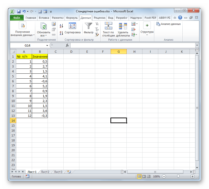
Для примера нами будет использована выборка из двенадцати чисел, представленных в таблице.
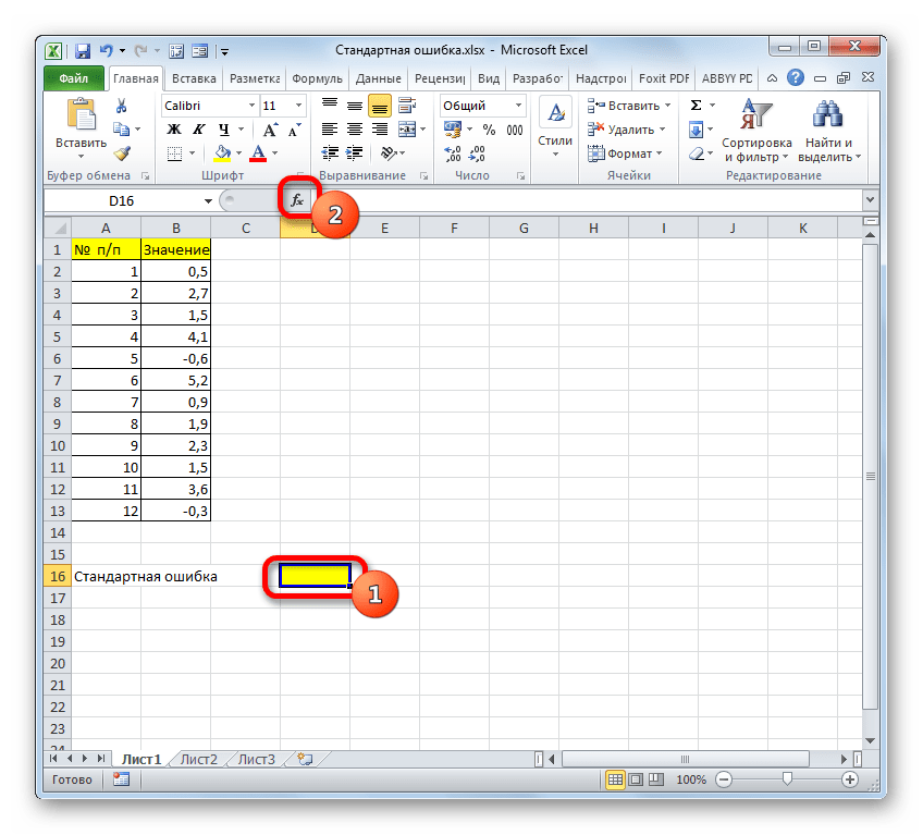
- Выделяем ячейку, в которой будет выводиться итоговое значение стандартной ошибки, и клацаем по иконке «Вставить функцию».
- Открывается Мастер функций. Производим перемещение в блок «Статистические». В представленном перечне наименований выбираем название «СТАНДОТКЛОН.В».
- Запускается окно аргументов вышеуказанного оператора. СТАНДОТКЛОН.В предназначен для оценивания стандартного отклонения при выборке. Данный оператор имеет следующий синтаксис:
=СТАНДОТКЛОН.В(число1;число2;…)«Число1» и последующие аргументы являются числовыми значениями или ссылками на ячейки и диапазоны листа, в которых они расположены. Всего может насчитываться до 255 аргументов этого типа. Обязательным является только первый аргумент.
Итак, устанавливаем курсор в поле «Число1». Далее, обязательно произведя зажим левой кнопки мыши, выделяем курсором весь диапазон выборки на листе. Координаты данного массива тут же отображаются в поле окна. После этого клацаем по кнопке «OK».
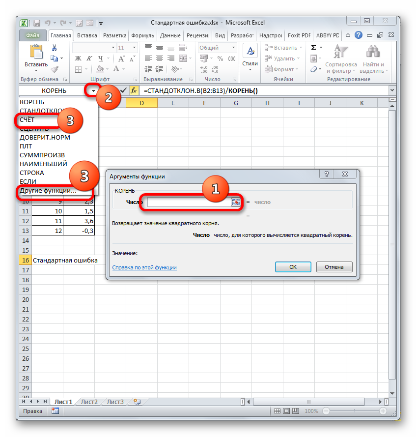
- В ячейку на листе выводится результат расчета оператора СТАНДОТКЛОН.В. Но это ещё не ошибка средней арифметической. Для того, чтобы получить искомое значение, нужно стандартное отклонение разделить на квадратный корень от количества элементов выборки. Для того, чтобы продолжить вычисления, выделяем ячейку, содержащую функцию СТАНДОТКЛОН.В. После этого устанавливаем курсор в строку формул и дописываем после уже существующего выражения знак деления (/). Вслед за этим клацаем по пиктограмме перевернутого вниз углом треугольника, которая располагается слева от строки формул. Открывается список недавно использованных функций. Если вы в нем найдете наименование оператора «КОРЕНЬ», то переходите по данному наименованию. В обратном случае жмите по пункту «Другие функции…».
- Снова происходит запуск Мастера функций. На этот раз нам следует посетить категорию «Математические». В представленном перечне выделяем название «КОРЕНЬ» и жмем на кнопку «OK».
- Открывается окно аргументов функции КОРЕНЬ. Единственной задачей данного оператора является вычисление квадратного корня из заданного числа. Его синтаксис предельно простой:
=КОРЕНЬ(число)
Как видим, функция имеет всего один аргумент «Число». Он может быть представлен числовым значением, ссылкой на ячейку, в которой оно содержится или другой функцией, вычисляющей это число. Последний вариант как раз и будет представлен в нашем примере.
Устанавливаем курсор в поле «Число» и кликаем по знакомому нам треугольнику, который вызывает список последних использованных функций. Ищем в нем наименование «СЧЁТ». Если находим, то кликаем по нему. В обратном случае, опять же, переходим по наименованию «Другие функции…».
- В раскрывшемся окне Мастера функций производим перемещение в группу «Статистические». Там выделяем наименование «СЧЁТ» и выполняем клик по кнопке «OK».
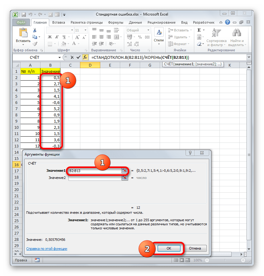
- Запускается окно аргументов функции СЧЁТ. Указанный оператор предназначен для вычисления количества ячеек, которые заполнены числовыми значениями. В нашем случае он будет подсчитывать количество элементов выборки и сообщать результат «материнскому» оператору КОРЕНЬ. Синтаксис функции следующий:
=СЧЁТ(значение1;значение2;…)В качестве аргументов «Значение», которых может насчитываться до 255 штук, выступают ссылки на диапазоны ячеек. Ставим курсор в поле «Значение1», зажимаем левую кнопку мыши и выделяем весь диапазон выборки. После того, как его координаты отобразились в поле, жмем на кнопку «OK».
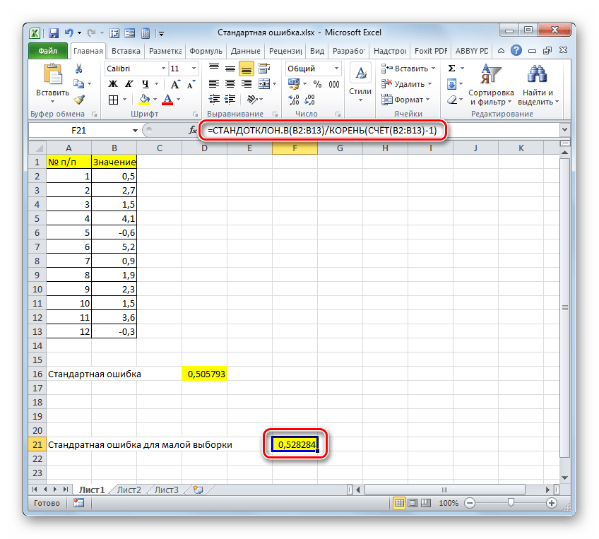
- После выполнения последнего действия будет не только рассчитано количество ячеек заполненных числами, но и вычислена ошибка средней арифметической, так как это был последний штрих в работе над данной формулой. Величина стандартной ошибки выведена в ту ячейку, где размещена сложная формула, общий вид которой в нашем случае следующий:
=СТАНДОТКЛОН.В(B2:B13)/КОРЕНЬ(СЧЁТ(B2:B13))Результат вычисления ошибки средней арифметической составил 0,505793. Запомним это число и сравним с тем, которое получим при решении поставленной задачи следующим способом.


Но дело в том, что для малых выборок (до 30 единиц) для большей точности лучше применять немного измененную формулу. В ней величина стандартного отклонения делится не на квадратный корень от количества элементов выборки, а на квадратный корень от количества элементов выборки минус один. Таким образом, с учетом нюансов малой выборки наша формула приобретет следующий вид:
=СТАНДОТКЛОН.В(B2:B13)/КОРЕНЬ(СЧЁТ(B2:B13)-1)
Урок: Статистические функции в Экселе
Способ 2: применение инструмента «Описательная статистика»
Вторым вариантом, с помощью которого можно вычислить стандартную ошибку в Экселе, является применение инструмента «Описательная статистика», входящего в набор инструментов «Анализ данных» («Пакет анализа»). «Описательная статистика» проводит комплексный анализ выборки по различным критериям. Одним из них как раз и является нахождение ошибки средней арифметической.
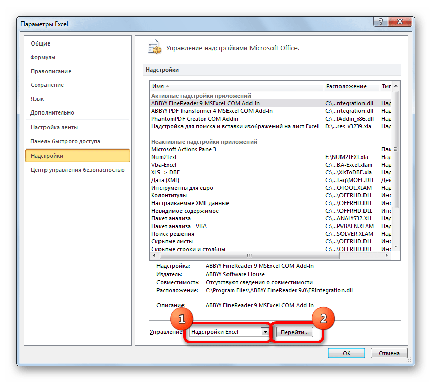
Но чтобы воспользоваться данной возможностью, нужно сразу активировать «Пакет анализа», так как по умолчанию в Экселе он отключен.
- После того, как открыт документ с выборкой, переходим во вкладку «Файл».
- Далее, воспользовавшись левым вертикальным меню, перемещаемся через его пункт в раздел «Параметры».
- Запускается окно параметров Эксель. В левой части данного окна размещено меню, через которое перемещаемся в подраздел «Надстройки».
- В самой нижней части появившегося окна расположено поле «Управление». Выставляем в нем параметр «Надстройки Excel» и жмем на кнопку «Перейти…» справа от него.
- Запускается окно надстроек с перечнем доступных скриптов. Отмечаем галочкой наименование «Пакет анализа» и щелкаем по кнопке «OK» в правой части окошка.
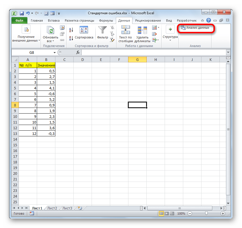
- После выполнения последнего действия на ленте появится новая группа инструментов, которая имеет наименование «Анализ». Чтобы перейти к ней, щелкаем по названию вкладки «Данные».
- После перехода жмем на кнопку «Анализ данных» в блоке инструментов «Анализ», который расположен в самом конце ленты.
- Запускается окошко выбора инструмента анализа. Выделяем наименование «Описательная статистика» и жмем на кнопку «OK» справа.
- Запускается окно настроек инструмента комплексного статистического анализа «Описательная статистика».
В поле «Входной интервал» необходимо указать диапазон ячеек таблицы, в которых находится анализируемая выборка. Вручную это делать неудобно, хотя и можно, поэтому ставим курсор в указанное поле и при зажатой левой кнопке мыши выделяем соответствующий массив данных на листе. Его координаты тут же отобразятся в поле окна.
В блоке «Группирование» оставляем настройки по умолчанию. То есть, переключатель должен стоять около пункта «По столбцам». Если это не так, то его следует переставить.
Галочку «Метки в первой строке» можно не устанавливать. Для решения нашего вопроса это не важно.
Далее переходим к блоку настроек «Параметры вывода». Здесь следует указать, куда именно будет выводиться результат расчета инструмента «Описательная статистика»:
- На новый лист;
- В новую книгу (другой файл);
- В указанный диапазон текущего листа.
Давайте выберем последний из этих вариантов. Для этого переставляем переключатель в позицию «Выходной интервал» и устанавливаем курсор в поле напротив данного параметра. После этого клацаем на листе по ячейке, которая станет верхним левым элементом массива вывода данных. Её координаты должны отобразиться в поле, в котором мы до этого устанавливали курсор.
Далее следует блок настроек определяющий, какие именно данные нужно вводить:
- Итоговая статистика;
- К-ый наибольший;
- К-ый наименьший;
- Уровень надежности.
Для определения стандартной ошибки обязательно нужно установить галочку около параметра «Итоговая статистика». Напротив остальных пунктов выставляем галочки на свое усмотрение. На решение нашей основной задачи это никак не повлияет.
После того, как все настройки в окне «Описательная статистика» установлены, щелкаем по кнопке «OK» в его правой части.
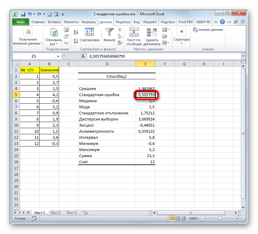
- После этого инструмент «Описательная статистика» выводит результаты обработки выборки на текущий лист. Как видим, это довольно много разноплановых статистических показателей, но среди них есть и нужный нам – «Стандартная ошибка». Он равен числу 0,505793. Это в точности тот же результат, который мы достигли путем применения сложной формулы при описании предыдущего способа.


Урок: Описательная статистика в Экселе
Как видим, в Экселе можно произвести расчет стандартной ошибки двумя способами: применив набор функций и воспользовавшись инструментом пакета анализа «Описательная статистика». Итоговый результат будет абсолютно одинаковый. Поэтому выбор метода зависит от удобства пользователя и поставленной конкретной задачи. Например, если ошибка средней арифметической является только одним из многих статистических показателей выборки, которые нужно рассчитать, то удобнее воспользоваться инструментом «Описательная статистика». Но если вам нужно вычислить исключительно этот показатель, то во избежание нагромождения лишних данных лучше прибегнуть к сложной формуле. В этом случае результат расчета уместится в одной ячейке листа.
In statistics, the mean squared error (MSE)[1] or mean squared deviation (MSD) of an estimator (of a procedure for estimating an unobserved quantity) measures the average of the squares of the errors—that is, the average squared difference between the estimated values and the actual value. MSE is a risk function, corresponding to the expected value of the squared error loss.[2] The fact that MSE is almost always strictly positive (and not zero) is because of randomness or because the estimator does not account for information that could produce a more accurate estimate.[3] In machine learning, specifically empirical risk minimization, MSE may refer to the empirical risk (the average loss on an observed data set), as an estimate of the true MSE (the true risk: the average loss on the actual population distribution).
The MSE is a measure of the quality of an estimator. As it is derived from the square of Euclidean distance, it is always a positive value that decreases as the error approaches zero.
The MSE is the second moment (about the origin) of the error, and thus incorporates both the variance of the estimator (how widely spread the estimates are from one data sample to another) and its bias (how far off the average estimated value is from the true value).[citation needed] For an unbiased estimator, the MSE is the variance of the estimator. Like the variance, MSE has the same units of measurement as the square of the quantity being estimated. In an analogy to standard deviation, taking the square root of MSE yields the root-mean-square error or root-mean-square deviation (RMSE or RMSD), which has the same units as the quantity being estimated; for an unbiased estimator, the RMSE is the square root of the variance, known as the standard error.
Definition and basic properties[edit]
The MSE either assesses the quality of a predictor (i.e., a function mapping arbitrary inputs to a sample of values of some random variable), or of an estimator (i.e., a mathematical function mapping a sample of data to an estimate of a parameter of the population from which the data is sampled). The definition of an MSE differs according to whether one is describing a predictor or an estimator.
Predictor[edit]
If a vector of 


In other words, the MSE is the mean 

In matrix notation,

where 


The MSE can also be computed on q data points that were not used in estimating the model, either because they were held back for this purpose, or because these data have been newly obtained. Within this process, known as statistical learning, the MSE is often called the test MSE,[4] and is computed as

Estimator[edit]
The MSE of an estimator 

![{displaystyle operatorname {MSE} ({hat {theta }})=operatorname {E} _{theta }left[({hat {theta }}-theta )^{2}right].}](https://wikimedia.org/api/rest_v1/media/math/render/svg/9a0e1b3bac58f9ba2d2f4ff8b85b2e35a8f4bf78)
This definition depends on the unknown parameter, but the MSE is a priori a property of an estimator. The MSE could be a function of unknown parameters, in which case any estimator of the MSE based on estimates of these parameters would be a function of the data (and thus a random variable). If the estimator
The MSE can be written as the sum of the variance of the estimator and the squared bias of the estimator, providing a useful way to calculate the MSE and implying that in the case of unbiased estimators, the MSE and variance are equivalent.[5]

Proof of variance and bias relationship[edit]
![{displaystyle {begin{aligned}operatorname {MSE} ({hat {theta }})&=operatorname {E} _{theta }left[({hat {theta }}-theta )^{2}right]\&=operatorname {E} _{theta }left[left({hat {theta }}-operatorname {E} _{theta }[{hat {theta }}]+operatorname {E} _{theta }[{hat {theta }}]-theta right)^{2}right]\&=operatorname {E} _{theta }left[left({hat {theta }}-operatorname {E} _{theta }[{hat {theta }}]right)^{2}+2left({hat {theta }}-operatorname {E} _{theta }[{hat {theta }}]right)left(operatorname {E} _{theta }[{hat {theta }}]-theta right)+left(operatorname {E} _{theta }[{hat {theta }}]-theta right)^{2}right]\&=operatorname {E} _{theta }left[left({hat {theta }}-operatorname {E} _{theta }[{hat {theta }}]right)^{2}right]+operatorname {E} _{theta }left[2left({hat {theta }}-operatorname {E} _{theta }[{hat {theta }}]right)left(operatorname {E} _{theta }[{hat {theta }}]-theta right)right]+operatorname {E} _{theta }left[left(operatorname {E} _{theta }[{hat {theta }}]-theta right)^{2}right]\&=operatorname {E} _{theta }left[left({hat {theta }}-operatorname {E} _{theta }[{hat {theta }}]right)^{2}right]+2left(operatorname {E} _{theta }[{hat {theta }}]-theta right)operatorname {E} _{theta }left[{hat {theta }}-operatorname {E} _{theta }[{hat {theta }}]right]+left(operatorname {E} _{theta }[{hat {theta }}]-theta right)^{2}&&operatorname {E} _{theta }[{hat {theta }}]-theta ={text{const.}}\&=operatorname {E} _{theta }left[left({hat {theta }}-operatorname {E} _{theta }[{hat {theta }}]right)^{2}right]+2left(operatorname {E} _{theta }[{hat {theta }}]-theta right)left(operatorname {E} _{theta }[{hat {theta }}]-operatorname {E} _{theta }[{hat {theta }}]right)+left(operatorname {E} _{theta }[{hat {theta }}]-theta right)^{2}&&operatorname {E} _{theta }[{hat {theta }}]={text{const.}}\&=operatorname {E} _{theta }left[left({hat {theta }}-operatorname {E} _{theta }[{hat {theta }}]right)^{2}right]+left(operatorname {E} _{theta }[{hat {theta }}]-theta right)^{2}\&=operatorname {Var} _{theta }({hat {theta }})+operatorname {Bias} _{theta }({hat {theta }},theta )^{2}end{aligned}}}](https://wikimedia.org/api/rest_v1/media/math/render/svg/2ac524a751828f971013e1297a33ca1cc4c38cd6)
An even shorter proof can be achieved using the well-known formula that for a random variable 


![{displaystyle {begin{aligned}operatorname {MSE} ({hat {theta }})&=mathbb {E} [({hat {theta }}-theta )^{2}]\&=operatorname {Var} ({hat {theta }}-theta )+(mathbb {E} [{hat {theta }}-theta ])^{2}\&=operatorname {Var} ({hat {theta }})+operatorname {Bias} ^{2}({hat {theta }})end{aligned}}}](https://wikimedia.org/api/rest_v1/media/math/render/svg/864646cf4426e2b62a3caf9460382eec1a77fe4e)
But in real modeling case, MSE could be described as the addition of model variance, model bias, and irreducible uncertainty (see Bias–variance tradeoff). According to the relationship, the MSE of the estimators could be simply used for the efficiency comparison, which includes the information of estimator variance and bias. This is called MSE criterion.
In regression[edit]
In regression analysis, plotting is a more natural way to view the overall trend of the whole data. The mean of the distance from each point to the predicted regression model can be calculated, and shown as the mean squared error. The squaring is critical to reduce the complexity with negative signs. To minimize MSE, the model could be more accurate, which would mean the model is closer to actual data. One example of a linear regression using this method is the least squares method—which evaluates appropriateness of linear regression model to model bivariate dataset,[6] but whose limitation is related to known distribution of the data.
The term mean squared error is sometimes used to refer to the unbiased estimate of error variance: the residual sum of squares divided by the number of degrees of freedom. This definition for a known, computed quantity differs from the above definition for the computed MSE of a predictor, in that a different denominator is used. The denominator is the sample size reduced by the number of model parameters estimated from the same data, (n−p) for p regressors or (n−p−1) if an intercept is used (see errors and residuals in statistics for more details).[7] Although the MSE (as defined in this article) is not an unbiased estimator of the error variance, it is consistent, given the consistency of the predictor.
In regression analysis, «mean squared error», often referred to as mean squared prediction error or «out-of-sample mean squared error», can also refer to the mean value of the squared deviations of the predictions from the true values, over an out-of-sample test space, generated by a model estimated over a particular sample space. This also is a known, computed quantity, and it varies by sample and by out-of-sample test space.
Examples[edit]
Mean[edit]
Suppose we have a random sample of size 


which has an expected value equal to the true mean
![{displaystyle operatorname {MSE} left({overline {X}}right)=operatorname {E} left[left({overline {X}}-mu right)^{2}right]=left({frac {sigma }{sqrt {n}}}right)^{2}={frac {sigma ^{2}}{n}}}](https://wikimedia.org/api/rest_v1/media/math/render/svg/b4647a2cc4c8f9a4c90b628faad2dcf80c4aae84)
where 
For a Gaussian distribution, this is the best unbiased estimator (i.e., one with the lowest MSE among all unbiased estimators), but not, say, for a uniform distribution.
Variance[edit]
The usual estimator for the variance is the corrected sample variance:

This is unbiased (its expected value is

where 

However, one can use other estimators for 

then we calculate:
![{displaystyle {begin{aligned}operatorname {MSE} (S_{a}^{2})&=operatorname {E} left[left({frac {n-1}{a}}S_{n-1}^{2}-sigma ^{2}right)^{2}right]\&=operatorname {E} left[{frac {(n-1)^{2}}{a^{2}}}S_{n-1}^{4}-2left({frac {n-1}{a}}S_{n-1}^{2}right)sigma ^{2}+sigma ^{4}right]\&={frac {(n-1)^{2}}{a^{2}}}operatorname {E} left[S_{n-1}^{4}right]-2left({frac {n-1}{a}}right)operatorname {E} left[S_{n-1}^{2}right]sigma ^{2}+sigma ^{4}\&={frac {(n-1)^{2}}{a^{2}}}operatorname {E} left[S_{n-1}^{4}right]-2left({frac {n-1}{a}}right)sigma ^{4}+sigma ^{4}&&operatorname {E} left[S_{n-1}^{2}right]=sigma ^{2}\&={frac {(n-1)^{2}}{a^{2}}}left({frac {gamma _{2}}{n}}+{frac {n+1}{n-1}}right)sigma ^{4}-2left({frac {n-1}{a}}right)sigma ^{4}+sigma ^{4}&&operatorname {E} left[S_{n-1}^{4}right]=operatorname {MSE} (S_{n-1}^{2})+sigma ^{4}\&={frac {n-1}{na^{2}}}left((n-1)gamma _{2}+n^{2}+nright)sigma ^{4}-2left({frac {n-1}{a}}right)sigma ^{4}+sigma ^{4}end{aligned}}}](https://wikimedia.org/api/rest_v1/media/math/render/svg/cf22322412b8454c706d78671e5d94208675a6e0)
This is minimized when

For a Gaussian distribution, where 


Further, while the corrected sample variance is the best unbiased estimator (minimum mean squared error among unbiased estimators) of variance for Gaussian distributions, if the distribution is not Gaussian, then even among unbiased estimators, the best unbiased estimator of the variance may not be 
Gaussian distribution[edit]
The following table gives several estimators of the true parameters of the population, μ and σ2, for the Gaussian case.[9]
| True value | Estimator | Mean squared error |
|---|---|---|
 |
= the unbiased estimator of the population mean,  |

|
 |
= the unbiased estimator of the population variance,  |

|
|
= the biased estimator of the population variance,  |

|
|
= the biased estimator of the population variance,  |

|
Interpretation[edit]
An MSE of zero, meaning that the estimator
Values of MSE may be used for comparative purposes. Two or more statistical models may be compared using their MSEs—as a measure of how well they explain a given set of observations: An unbiased estimator (estimated from a statistical model) with the smallest variance among all unbiased estimators is the best unbiased estimator or MVUE (Minimum-Variance Unbiased Estimator).
Both analysis of variance and linear regression techniques estimate the MSE as part of the analysis and use the estimated MSE to determine the statistical significance of the factors or predictors under study. The goal of experimental design is to construct experiments in such a way that when the observations are analyzed, the MSE is close to zero relative to the magnitude of at least one of the estimated treatment effects.
In one-way analysis of variance, MSE can be calculated by the division of the sum of squared errors and the degree of freedom. Also, the f-value is the ratio of the mean squared treatment and the MSE.
MSE is also used in several stepwise regression techniques as part of the determination as to how many predictors from a candidate set to include in a model for a given set of observations.
Applications[edit]
- Minimizing MSE is a key criterion in selecting estimators: see minimum mean-square error. Among unbiased estimators, minimizing the MSE is equivalent to minimizing the variance, and the estimator that does this is the minimum variance unbiased estimator. However, a biased estimator may have lower MSE; see estimator bias.
- In statistical modelling the MSE can represent the difference between the actual observations and the observation values predicted by the model. In this context, it is used to determine the extent to which the model fits the data as well as whether removing some explanatory variables is possible without significantly harming the model’s predictive ability.
- In forecasting and prediction, the Brier score is a measure of forecast skill based on MSE.
Loss function[edit]
Squared error loss is one of the most widely used loss functions in statistics[citation needed], though its widespread use stems more from mathematical convenience than considerations of actual loss in applications. Carl Friedrich Gauss, who introduced the use of mean squared error, was aware of its arbitrariness and was in agreement with objections to it on these grounds.[3] The mathematical benefits of mean squared error are particularly evident in its use at analyzing the performance of linear regression, as it allows one to partition the variation in a dataset into variation explained by the model and variation explained by randomness.
Criticism[edit]
The use of mean squared error without question has been criticized by the decision theorist James Berger. Mean squared error is the negative of the expected value of one specific utility function, the quadratic utility function, which may not be the appropriate utility function to use under a given set of circumstances. There are, however, some scenarios where mean squared error can serve as a good approximation to a loss function occurring naturally in an application.[10]
Like variance, mean squared error has the disadvantage of heavily weighting outliers.[11] This is a result of the squaring of each term, which effectively weights large errors more heavily than small ones. This property, undesirable in many applications, has led researchers to use alternatives such as the mean absolute error, or those based on the median.
See also[edit]
- Bias–variance tradeoff
- Hodges’ estimator
- James–Stein estimator
- Mean percentage error
- Mean square quantization error
- Mean square weighted deviation
- Mean squared displacement
- Mean squared prediction error
- Minimum mean square error
- Minimum mean squared error estimator
- Overfitting
- Peak signal-to-noise ratio
Notes[edit]
- ^ This can be proved by Jensen’s inequality as follows. The fourth central moment is an upper bound for the square of variance, so that the least value for their ratio is one, therefore, the least value for the excess kurtosis is −2, achieved, for instance, by a Bernoulli with p=1/2.
References[edit]
- ^ a b «Mean Squared Error (MSE)». www.probabilitycourse.com. Retrieved 2020-09-12.
- ^ Bickel, Peter J.; Doksum, Kjell A. (2015). Mathematical Statistics: Basic Ideas and Selected Topics. Vol. I (Second ed.). p. 20.
If we use quadratic loss, our risk function is called the mean squared error (MSE) …
- ^ a b Lehmann, E. L.; Casella, George (1998). Theory of Point Estimation (2nd ed.). New York: Springer. ISBN 978-0-387-98502-2. MR 1639875.
- ^ Gareth, James; Witten, Daniela; Hastie, Trevor; Tibshirani, Rob (2021). An Introduction to Statistical Learning: with Applications in R. Springer. ISBN 978-1071614174.
- ^ Wackerly, Dennis; Mendenhall, William; Scheaffer, Richard L. (2008). Mathematical Statistics with Applications (7 ed.). Belmont, CA, USA: Thomson Higher Education. ISBN 978-0-495-38508-0.
- ^ A modern introduction to probability and statistics : understanding why and how. Dekking, Michel, 1946-. London: Springer. 2005. ISBN 978-1-85233-896-1. OCLC 262680588.
{{cite book}}: CS1 maint: others (link) - ^ Steel, R.G.D, and Torrie, J. H., Principles and Procedures of Statistics with Special Reference to the Biological Sciences., McGraw Hill, 1960, page 288.
- ^ Mood, A.; Graybill, F.; Boes, D. (1974). Introduction to the Theory of Statistics (3rd ed.). McGraw-Hill. p. 229.
- ^ DeGroot, Morris H. (1980). Probability and Statistics (2nd ed.). Addison-Wesley.
- ^ Berger, James O. (1985). «2.4.2 Certain Standard Loss Functions». Statistical Decision Theory and Bayesian Analysis (2nd ed.). New York: Springer-Verlag. p. 60. ISBN 978-0-387-96098-2. MR 0804611.
- ^ Bermejo, Sergio; Cabestany, Joan (2001). «Oriented principal component analysis for large margin classifiers». Neural Networks. 14 (10): 1447–1461. doi:10.1016/S0893-6080(01)00106-X. PMID 11771723.
In statistics, the mean squared error (MSE)[1] or mean squared deviation (MSD) of an estimator (of a procedure for estimating an unobserved quantity) measures the average of the squares of the errors—that is, the average squared difference between the estimated values and the actual value. MSE is a risk function, corresponding to the expected value of the squared error loss.[2] The fact that MSE is almost always strictly positive (and not zero) is because of randomness or because the estimator does not account for information that could produce a more accurate estimate.[3] In machine learning, specifically empirical risk minimization, MSE may refer to the empirical risk (the average loss on an observed data set), as an estimate of the true MSE (the true risk: the average loss on the actual population distribution).
The MSE is a measure of the quality of an estimator. As it is derived from the square of Euclidean distance, it is always a positive value that decreases as the error approaches zero.
The MSE is the second moment (about the origin) of the error, and thus incorporates both the variance of the estimator (how widely spread the estimates are from one data sample to another) and its bias (how far off the average estimated value is from the true value).[citation needed] For an unbiased estimator, the MSE is the variance of the estimator. Like the variance, MSE has the same units of measurement as the square of the quantity being estimated. In an analogy to standard deviation, taking the square root of MSE yields the root-mean-square error or root-mean-square deviation (RMSE or RMSD), which has the same units as the quantity being estimated; for an unbiased estimator, the RMSE is the square root of the variance, known as the standard error.
Definition and basic properties[edit]
The MSE either assesses the quality of a predictor (i.e., a function mapping arbitrary inputs to a sample of values of some random variable), or of an estimator (i.e., a mathematical function mapping a sample of data to an estimate of a parameter of the population from which the data is sampled). The definition of an MSE differs according to whether one is describing a predictor or an estimator.
Predictor[edit]
If a vector of
In other words, the MSE is the mean
In matrix notation,
where
The MSE can also be computed on q data points that were not used in estimating the model, either because they were held back for this purpose, or because these data have been newly obtained. Within this process, known as statistical learning, the MSE is often called the test MSE,[4] and is computed as
Estimator[edit]
The MSE of an estimator
This definition depends on the unknown parameter, but the MSE is a priori a property of an estimator. The MSE could be a function of unknown parameters, in which case any estimator of the MSE based on estimates of these parameters would be a function of the data (and thus a random variable). If the estimator
The MSE can be written as the sum of the variance of the estimator and the squared bias of the estimator, providing a useful way to calculate the MSE and implying that in the case of unbiased estimators, the MSE and variance are equivalent.[5]
Proof of variance and bias relationship[edit]
An even shorter proof can be achieved using the well-known formula that for a random variable
But in real modeling case, MSE could be described as the addition of model variance, model bias, and irreducible uncertainty (see Bias–variance tradeoff). According to the relationship, the MSE of the estimators could be simply used for the efficiency comparison, which includes the information of estimator variance and bias. This is called MSE criterion.
In regression[edit]
In regression analysis, plotting is a more natural way to view the overall trend of the whole data. The mean of the distance from each point to the predicted regression model can be calculated, and shown as the mean squared error. The squaring is critical to reduce the complexity with negative signs. To minimize MSE, the model could be more accurate, which would mean the model is closer to actual data. One example of a linear regression using this method is the least squares method—which evaluates appropriateness of linear regression model to model bivariate dataset,[6] but whose limitation is related to known distribution of the data.
The term mean squared error is sometimes used to refer to the unbiased estimate of error variance: the residual sum of squares divided by the number of degrees of freedom. This definition for a known, computed quantity differs from the above definition for the computed MSE of a predictor, in that a different denominator is used. The denominator is the sample size reduced by the number of model parameters estimated from the same data, (n−p) for p regressors or (n−p−1) if an intercept is used (see errors and residuals in statistics for more details).[7] Although the MSE (as defined in this article) is not an unbiased estimator of the error variance, it is consistent, given the consistency of the predictor.
In regression analysis, «mean squared error», often referred to as mean squared prediction error or «out-of-sample mean squared error», can also refer to the mean value of the squared deviations of the predictions from the true values, over an out-of-sample test space, generated by a model estimated over a particular sample space. This also is a known, computed quantity, and it varies by sample and by out-of-sample test space.
Examples[edit]
Mean[edit]
Suppose we have a random sample of size
which has an expected value equal to the true mean
where
For a Gaussian distribution, this is the best unbiased estimator (i.e., one with the lowest MSE among all unbiased estimators), but not, say, for a uniform distribution.
Variance[edit]
The usual estimator for the variance is the corrected sample variance:
This is unbiased (its expected value is
where
However, one can use other estimators for
then we calculate:
This is minimized when
For a Gaussian distribution, where
Further, while the corrected sample variance is the best unbiased estimator (minimum mean squared error among unbiased estimators) of variance for Gaussian distributions, if the distribution is not Gaussian, then even among unbiased estimators, the best unbiased estimator of the variance may not be
Gaussian distribution[edit]
The following table gives several estimators of the true parameters of the population, μ and σ2, for the Gaussian case.[9]
| True value | Estimator | Mean squared error |
|---|---|---|
|
= the unbiased estimator of the population mean, |
|
|
= the unbiased estimator of the population variance, |
|
|
= the biased estimator of the population variance, |
|
|
= the biased estimator of the population variance, |
|
Interpretation[edit]
An MSE of zero, meaning that the estimator
Values of MSE may be used for comparative purposes. Two or more statistical models may be compared using their MSEs—as a measure of how well they explain a given set of observations: An unbiased estimator (estimated from a statistical model) with the smallest variance among all unbiased estimators is the best unbiased estimator or MVUE (Minimum-Variance Unbiased Estimator).
Both analysis of variance and linear regression techniques estimate the MSE as part of the analysis and use the estimated MSE to determine the statistical significance of the factors or predictors under study. The goal of experimental design is to construct experiments in such a way that when the observations are analyzed, the MSE is close to zero relative to the magnitude of at least one of the estimated treatment effects.
In one-way analysis of variance, MSE can be calculated by the division of the sum of squared errors and the degree of freedom. Also, the f-value is the ratio of the mean squared treatment and the MSE.
MSE is also used in several stepwise regression techniques as part of the determination as to how many predictors from a candidate set to include in a model for a given set of observations.
Applications[edit]
- Minimizing MSE is a key criterion in selecting estimators: see minimum mean-square error. Among unbiased estimators, minimizing the MSE is equivalent to minimizing the variance, and the estimator that does this is the minimum variance unbiased estimator. However, a biased estimator may have lower MSE; see estimator bias.
- In statistical modelling the MSE can represent the difference between the actual observations and the observation values predicted by the model. In this context, it is used to determine the extent to which the model fits the data as well as whether removing some explanatory variables is possible without significantly harming the model’s predictive ability.
- In forecasting and prediction, the Brier score is a measure of forecast skill based on MSE.
Loss function[edit]
Squared error loss is one of the most widely used loss functions in statistics[citation needed], though its widespread use stems more from mathematical convenience than considerations of actual loss in applications. Carl Friedrich Gauss, who introduced the use of mean squared error, was aware of its arbitrariness and was in agreement with objections to it on these grounds.[3] The mathematical benefits of mean squared error are particularly evident in its use at analyzing the performance of linear regression, as it allows one to partition the variation in a dataset into variation explained by the model and variation explained by randomness.
Criticism[edit]
The use of mean squared error without question has been criticized by the decision theorist James Berger. Mean squared error is the negative of the expected value of one specific utility function, the quadratic utility function, which may not be the appropriate utility function to use under a given set of circumstances. There are, however, some scenarios where mean squared error can serve as a good approximation to a loss function occurring naturally in an application.[10]
Like variance, mean squared error has the disadvantage of heavily weighting outliers.[11] This is a result of the squaring of each term, which effectively weights large errors more heavily than small ones. This property, undesirable in many applications, has led researchers to use alternatives such as the mean absolute error, or those based on the median.
See also[edit]
- Bias–variance tradeoff
- Hodges’ estimator
- James–Stein estimator
- Mean percentage error
- Mean square quantization error
- Mean square weighted deviation
- Mean squared displacement
- Mean squared prediction error
- Minimum mean square error
- Minimum mean squared error estimator
- Overfitting
- Peak signal-to-noise ratio
Notes[edit]
- ^ This can be proved by Jensen’s inequality as follows. The fourth central moment is an upper bound for the square of variance, so that the least value for their ratio is one, therefore, the least value for the excess kurtosis is −2, achieved, for instance, by a Bernoulli with p=1/2.
References[edit]
- ^ a b «Mean Squared Error (MSE)». www.probabilitycourse.com. Retrieved 2020-09-12.
- ^ Bickel, Peter J.; Doksum, Kjell A. (2015). Mathematical Statistics: Basic Ideas and Selected Topics. Vol. I (Second ed.). p. 20.
If we use quadratic loss, our risk function is called the mean squared error (MSE) …
- ^ a b Lehmann, E. L.; Casella, George (1998). Theory of Point Estimation (2nd ed.). New York: Springer. ISBN 978-0-387-98502-2. MR 1639875.
- ^ Gareth, James; Witten, Daniela; Hastie, Trevor; Tibshirani, Rob (2021). An Introduction to Statistical Learning: with Applications in R. Springer. ISBN 978-1071614174.
- ^ Wackerly, Dennis; Mendenhall, William; Scheaffer, Richard L. (2008). Mathematical Statistics with Applications (7 ed.). Belmont, CA, USA: Thomson Higher Education. ISBN 978-0-495-38508-0.
- ^ A modern introduction to probability and statistics : understanding why and how. Dekking, Michel, 1946-. London: Springer. 2005. ISBN 978-1-85233-896-1. OCLC 262680588.
{{cite book}}: CS1 maint: others (link) - ^ Steel, R.G.D, and Torrie, J. H., Principles and Procedures of Statistics with Special Reference to the Biological Sciences., McGraw Hill, 1960, page 288.
- ^ Mood, A.; Graybill, F.; Boes, D. (1974). Introduction to the Theory of Statistics (3rd ed.). McGraw-Hill. p. 229.
- ^ DeGroot, Morris H. (1980). Probability and Statistics (2nd ed.). Addison-Wesley.
- ^ Berger, James O. (1985). «2.4.2 Certain Standard Loss Functions». Statistical Decision Theory and Bayesian Analysis (2nd ed.). New York: Springer-Verlag. p. 60. ISBN 978-0-387-96098-2. MR 0804611.
- ^ Bermejo, Sergio; Cabestany, Joan (2001). «Oriented principal component analysis for large margin classifiers». Neural Networks. 14 (10): 1447–1461. doi:10.1016/S0893-6080(01)00106-X. PMID 11771723.
2.1. Стандартное отклонение среднего выборочного значения (ошибка среднего) и доверительный интервал
Результаты измерений обычно показывают с так называемой «средней статистической ошибкой средней величины» и для нашего случая (см. табл. 1.1) это будет запись: «высота сеянцев в опыте составила 5,0 ± 0,28 см». Словосочетание «средняя статистическая ошибка» обычно сокращают до названия «ошибка среднего» или просто «ошибка», обозначают буквой m и определяют по очень простой формуле. Для итогов упомянутой таблицы, где расчеты по 25 высотам дали значение δ = 1,42 см, эта ошибка составит:
 (2.1)
(2.1)
|
где δ – |
стандартное отклонение; |
|
N – |
число наблюдений или объем выборки, шт. |
Если объем выборки взять 100 шт., то ошибка снизится в 2 раза:  а если увеличить до 10000 шт., то в 10 раз, до 0,014 см.
Рассмотрим эту «среднюю статистическую ошибку» (далее просто ошибка) подробно, так как именно в ней скрыто понимание того, что называют статистическим мышлением. Интуитивно мы понимаем, что малая выборка дает большую ошибку, т.е. неточное определение среднего значения. Последний термин настолько привычен, что мы даже не задумываемся о том, что его правильное и полное название «среднее выборочное значение», т.е. среднее, определяемое в некоторой выборке. И выборки могут быть очень разные по численности. Начнем с самых малых. Например, что произойдет с ошибкой, если объем выборки сократить до 2 измерений? Такие выборки бывают, например, в почвенных исследованиях, когда каждое измерение достается дорогой ценой. Для этого вернемся к рис. 1.1. На нем стандартное отклонение ±δ, которое отражает разброс значений вокруг среднего в левую и правую сторону в виде холма, наблюдается при объеме выборки 1 шт. В этом случае ошибка среднего выборочного значения будет равна стандартному отклонению: m = δ = 1,42. С увеличением N ошибка уменьшается:
при объеме выборки N = 2 ошибка будет
при объеме выборки N = 4 ошибка будет
при объеме выборки N = 16 ошибка будет
Важно понять, что ряд распределения частот этих выборочных средних будет постепенно как бы съеживаться и приближаться к центру, где находится так называемое «генеральное» среднее. Поясним, что в математике генеральное среднее значение называется математическим ожиданием и его обозначают буквой «М». Например, это может быть средняя высота, рассчитанная по всем измеренным в теплице сеянцам, или среднее число семян в 1 шишке у дерева после подсчета семян во всех собранных с дерева шишках (50, 100, 500 и т.д., т.е. весьма небольшая генеральная совокупность). Распределение частот значений выборочных средних, которых может быть множество, будет иметь форму такого же холма, как и распределение единичных значений на рис. 1.1. При этом, если выборка будет из 1 шт., то холм будет в точности таким же, но при выборках из 2 шт. его форма съежится в  = в 1,41 раза; при выборках из 4 шт. –
в  = в 2 раза; при выборках из 9 шт. – в
  = в 3 раза и т.д.
Для этих сокращающихся рядов распределения выборочных средних можно рассчитать свое, особое стандартное отклонение. Вероятно, чтобы не путать его со СТАНДОТКЛ, его стали называть по-другому, т.е. «средней статистической ошибкой средней величины». Чем больше по объему выборки, тем короче ряд распределения средних значений этих выборок с его «хвостами» в левую и правую сторону, и тем меньше величина этого особого стандартного отклонения. Закон распределения частот выборочных средних точно такой же, и имеет те же свойства: в пределах ±2m находится 95 % всех значений выборочных средних, в пределах ±3m – 99,5 %, а в пределах ±4m находится 100 % всех значений xср. Форма этого распределения меняется от пологой при малых выборках до очень крутой, вплоть до «схлопывания» в центре при выборках большого объема, когда ошибка среднего стремится к нулю.
Здесь следует пояснить, что, на наш взгляд, словосочетание «средняя статистическая ошибка средней величины», сокращаемое до «ошибки среднего значения» или просто до «ошибки», вводит нас в некоторое заблуждение, так как мы привыкли со школы, что ошибки надобно исправлять. Более правильным, вместо слов «ошибка среднего значения», будет использование слов «стандартное отклонение выборочных средних значений от генерального среднего». Не случайно математики выбрали для обозначения величины этого отклонения букву «m», а для обозначения генерального среднего (математического ожидания) – букву «М». Слова для объяснения этих сложных явлений могут быть разными, но и у математиков, и у биологов есть единодушие в понимании статистического смысла, лежащего за этими буквенными символами. Вообще, лучше было бы ввести некий иной термин вместо слов «ошибка» или «отклонение», так как они изначально имеют в нашем сознании иной смысл; на наш взгляд, более всего подходит слово «скачок» (чем сильнее отскакивает выборочное среднее от генерального среднего, тем реже оно встречается). Но так уж получилось, что не нашлось нейтрального (иностранного) слова, и слово «ошибка» традиционно используют, и мы также будем его использовать; важно понимать его иной, чем в обыденном употреблении, математический и статистический смысл.
Для самого точного определения средней высоты сеянцев нужно измерять все растения в питомнике, и тогда мы получим «генеральное среднее значение». Но так не делают, а измеряют несколько сотен растений в разных местах и этого бывает достаточно для определения среднего выборочного значения с приемлемой точностью. В нашем примере при 100 растениях ошибка его определения составит  а ее отнесение к средней высоте сеянцев 5,0 см, выражаемое в %, дает нам так называемую точность опыта: 0,14/5,0×100 = 2,8 %. В биологии точность опыта ±2–3 % считается высокой, ±5 % – достаточной, а ±6–7 % – пониженной, но это весьма упрощенное представление о планировании эксперимента.
Вообще, точность опыта не самоцель; гораздо важнее сократить численность (объем) выборки до минимума. Представим себе, что средняя высота сеянцев xср = 5,0 см, а ее ±δ = 1,42 см, рассмотренные выше, получены при измерении 1000 растений потомства сосны, например, из Кунгура. Поделив ±δ на корень из 1000 получаем ошибку опыта m = ±0,045 см. Далее получаем точность опыта
Р = m/xср×100 = 0,045/5,0×100 = 0,9 %.
Точность получилась очень высокой. Но в питомнике есть потомства и из других мест и такой уровень точности совершенно не нужен, так как нужно узнать еще высоты сеянцев, например, из Очера, Осы, Добрянки и других районов. Если выборку из 1 тыс. растений снижать, то будет увеличиваться ошибка в определении средней высоты. И нужно найти приемлемую величину такой ошибки, которая позволит нам, тем не менее, уверенно утверждать, что это потомство растет быстрее, либо медленнее других. Причем происхождений может быть несколько сотен и минимизация выборок крайне важна, так как масштабы работ ограничены физическими возможностями бригады селекционеров. Следовательно, надо сокращать объем выборки. Как это сделать правильно?
Рассмотрим два потомства. Первое – это упомянутые сеянцы происхождением из Кунгура (хср1), второе – сеянцы из Кизела с хср2 = 6,0 см и δ2 = ± 1,0 см (превышение высоты на 20 %). Надо это превышение доказать. При выборках из 100 растений ранее определенная ошибка m1 была равна 0,14 см, вторая ошибка m2 после расчетов по формуле (2.1) составит 0,1 см. По закону нормального распределения 99,5 % всех возможных значений этих средних хср1 и хср2 будут в пределах «плюс-минус три ошибки», что можно показать графически (рис. 2.1) или в виде формул:
хср1 ± 3m1 = 5,0 ± 3×0,14 = 5,0 ± 0,4 см
и
хср2 ± 3m2 = 6,0 ± 3×0,1 = 6,0 ± 0,3 см.
Возможные теоретические значения средних в генеральной совокупности не перекрывают друг друга, значит, различие достоверно. А если сократить выборки до 50 сеянцев? Тогда 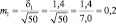 и
и  и пределы колебаний возможных значений средних будут:
хср1 ± 3m1 = 5,0 ± 3×0,20 = 5,0 ± 0,6 см;
хср2 ± 3m2 = 6,0 ± 3×0,14 = 6,0 ± 0,3 см.
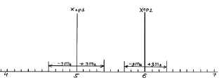
Рис. 2.1. Средние значения по выборкам из 100 растений и их тройные ошибки (пределы возможных значений выборочных средних в 99,5 % случаев)
Снова вынесем эти пределы на график (рис. 2.2).
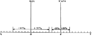
Рис. 2.2. Средние значения при N = 50 растений и их тройные ошибки
Как видим, пределы сблизились и если еще сократить выборки, то они перекроются. Можно ли далее снижать объем выборки?
Можно, но здесь вступает в силу так называемое условие безошибочного прогноза. Мы это условие задали на уровне 99,5 % и для этого взяли ±3m для распределения ошибок. Но можно взять уровень пониже, с пределами ±2δ (уровень 95 %) и даже с пределами ±1,7δ (уровень 90 %).
При выборках из 25 штук сеянцев, получаем две ошибки: 
 Тогда пределы значений для этих двух выборочных средних для уровня прогноза в 95 % будут:
хср1 ± 2m1 = 5,0 ± 2×0,28 = 5,0 ± 0,56 см;
хср2 ± 2m2 = 6,0 ± 2×0,20 = 6,0 ± 0,40 см.
Выносим эти пределы опять на график (рис. 2.3).
Рис. 2.3. Средние значения при N = 25 растений и их двойные ошибки (пределы возможных значений средних в 95 % случаев)
Как видим, просвет все еще есть, и поэтому между возможными значениями средних высот сеянцев в других выборках из происхождений Кунгур и Кизел различия будут опять доказаны. Но уровень доказательства понизился до 95 %, и для 5 % оставшихся случаев нет гарантии, что различия будут иметь место при выборке из 25 растений. Их может и не быть, но эту вероятность в 5 % мы допускаем.
Чтобы
судить о том, насколько точно проведенные
измерения отражают состав генеральной
совокупности, необходимо вычислить
стандартную ошибку средней арифметической
выборочной совокупности.
Стандартная
ошибка средней арифметической
характеризует степень отклонения
выборочной средней арифметической от
средней арифметической генеральной
совокупности.
Стандартная
ошибка средней арифметической вычисляется
по формуле:
![]() ,
,
где
– стандартное отклонение результатов
измерений, n
– объем выборки.
Зачастую
мы имеем дело с одной случайной выборкой
и с одной полученной при ее обработке
выборочной средней. Задача заключается
в суждении о величине неизвестной
генеральной средней по полученной
неточной величине случайной выборочной
средней.
Вычислим
среднюю ошибку найденного выборочного
среднего значения роста:
![]() 195
195
см; σ = 8,8 см;
![]() см.
см.
2,8 см
составляют не максимальную, а среднюю
возможную ошибку среднего. Отдельные
выборочные средние могут отклоняться
от генеральной как больше, так и меньше,
чем на 2,8 см.
Каковы
же пределы возможных ошибок случайной
выборки, какова ее максимальная ошибка?
Величина максимальной ошибки зависит
от величины средней ошибки и вычисляется
по формуле
![]() .
.
При
объеме выборки n
= 10:
![]() .
.
Все
случайные выборочные средние, которые
могут быть получены в подобных опытах
(в том числе и фактически полученная
выборочная средняя
![]() = 195 см), при своем варьировании около
= 195 см), при своем варьировании около
неизвестного генерального среднего в
подавляющем количестве группируются
около него так, что лишь ничтожный
процент их отклоняется от генеральной
средней более, чем на величину максимальной
ошибки.
Другими
словами, генеральная средняя определяется
как
![]() .
.
Эти пределы
колебаний значительно сужаются, если
средняя ошибка уменьшается благодаря
увеличению численности выборки.
Искомая
генеральная средняя лежит между
![]() и
и![]() .
.
Таким образом, при высокой точности
выполнения эксперимента и достаточно
большом числе измерений можно определить
среднюю арифметическую бесконечно
большого числа экспериментов.
До сих
пор мы определяли максимальную ошибку
выборочной средней, исходя из того, что
все остальные показатели известны. Если
же мы хотим достичь определенной
точности, определенного приближения к
генеральной средней, в этом случае
встает вопрос о численности выборки (о
том, сколько измерений, опытов необходимо
провести).
Допустим, что
максимальная ошибка должна быть равна
5 см. Сколько человек надо обследовать
(измерить) в нашем случае?
![]() .
.
Следовательно,
мы должны провести измерения роста у
36 баскетболистов высокого класса.
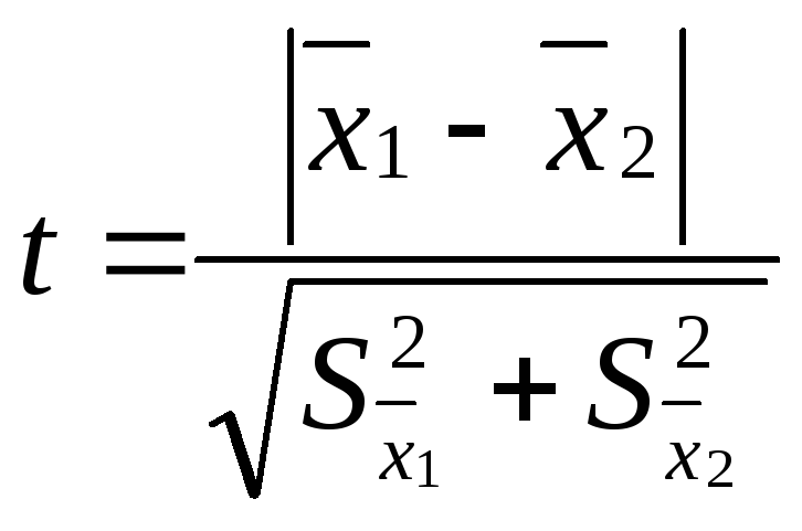
10. Достоверность различий
Следующим
важным вопросом практически для каждого
экспериментатора является умение
доказать достоверность различий между
двумя рядами признаков.
Проверку
достоверности различия двух рядов
измерений производят путем вычисления
критерия достоверности различия – t:
 ,
,
где
![]() – средняя одной выборки;
– средняя одной выборки;![]() – средняя другой выборки;
– средняя другой выборки;![]() – средняя ошибка первой выборки;
– средняя ошибка первой выборки;![]() – второй выборки. Если t < 2, то различие
– второй выборки. Если t < 2, то различие
между двумя выборками считается
недостоверным, если t
2, то различие между двумя выборками
достоверно на 95%.
Соседние файлы в предмете [НЕСОРТИРОВАННОЕ]
- #
- #
- #
- #
- #
- #
- #
- #
- #
- #
- #
17 авг. 2022 г.
читать 2 мин
Стандартная ошибка среднего — это способ измерить, насколько разбросаны значения в наборе данных. Он рассчитывается как:
Стандартная ошибка = с / √n
куда:
- s : стандартное отклонение выборки
- n : размер выборки
Вы можете рассчитать стандартную ошибку среднего для любого набора данных в Excel, используя следующую формулу:
= СТАНДОТКЛОН (диапазон значений) / КОРЕНЬ ( СЧЁТ (диапазон значений))
В следующем примере показано, как использовать эту формулу.
Пример: Стандартная ошибка в Excel
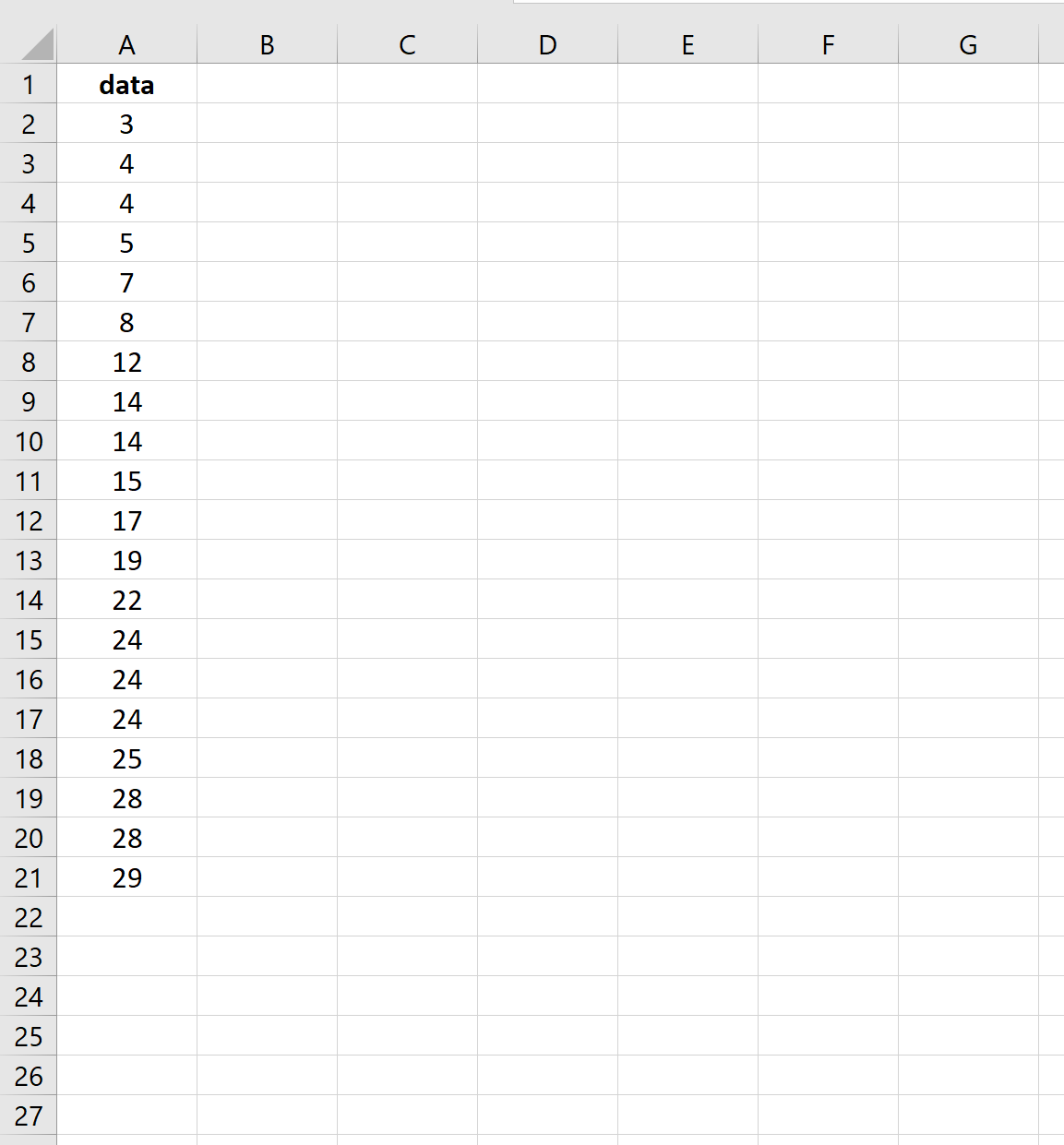
Предположим, у нас есть следующий набор данных:
На следующем снимке экрана показано, как рассчитать стандартную ошибку среднего значения для этого набора данных:
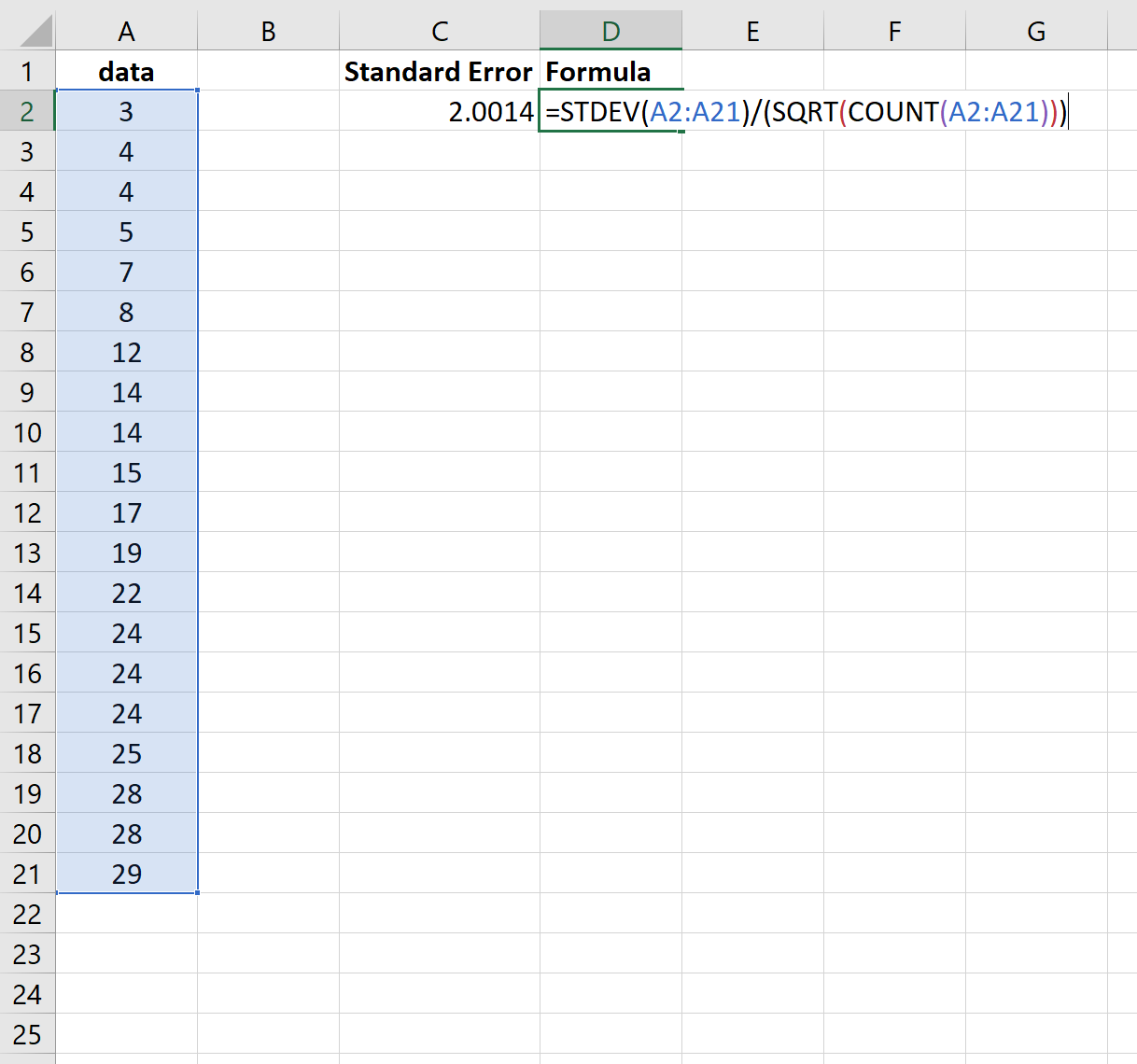
Стандартная ошибка оказывается равной 2,0014 .
Обратите внимание, что функция =СТАНДОТКЛОН() вычисляет выборочное среднее, что эквивалентно функции =СТАНДОТКЛОН.С() в Excel.
Таким образом, мы могли бы использовать следующую формулу для получения тех же результатов:

И снова стандартная ошибка оказывается равной 2,0014 .
Как интерпретировать стандартную ошибку среднего
Стандартная ошибка среднего — это просто мера того, насколько разбросаны значения вокруг среднего. При интерпретации стандартной ошибки среднего следует помнить о двух вещах:
1. Чем больше стандартная ошибка среднего, тем более разбросаны значения вокруг среднего в наборе данных.
Чтобы проиллюстрировать это, рассмотрим, изменим ли мы последнее значение в предыдущем наборе данных на гораздо большее число:
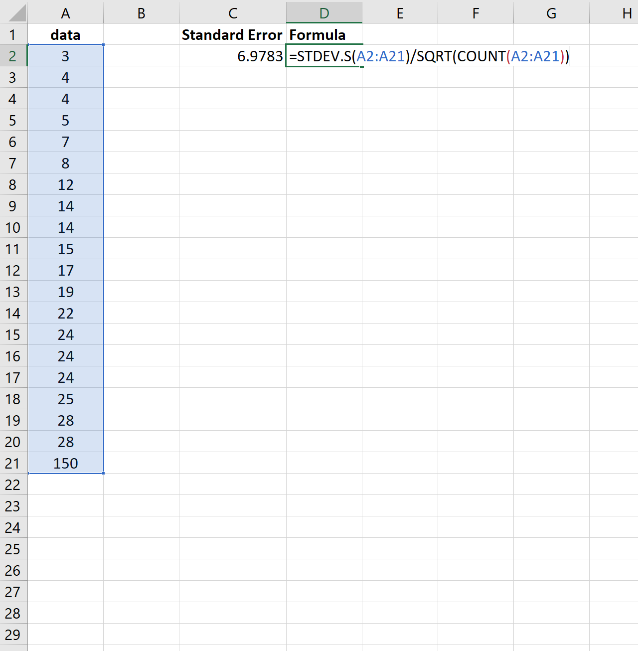
Обратите внимание на скачок стандартной ошибки с 2,0014 до 6,9783.Это указывает на то, что значения в этом наборе данных более разбросаны вокруг среднего значения по сравнению с предыдущим набором данных.
2. По мере увеличения размера выборки стандартная ошибка среднего имеет тенденцию к уменьшению.
Чтобы проиллюстрировать это, рассмотрим стандартную ошибку среднего для следующих двух наборов данных:
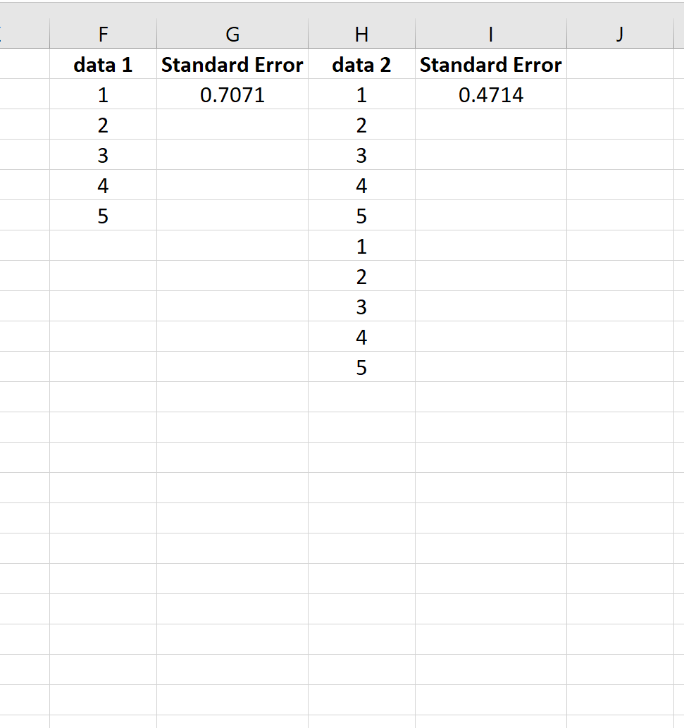
Второй набор данных — это просто первый набор данных, повторенный дважды. Таким образом, два набора данных имеют одинаковое среднее значение, но второй набор данных имеет больший размер выборки, поэтому стандартная ошибка меньше.