Доверительная вероятность р 95 означает что риск допустить ошибку составляет не более

Р=0,95

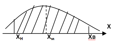
В
основе этой операции лежит оценка
принадлежности результатов измерения
к области безопасных значений (D).
При использовании доверительного
интервала заранее оговаривается желаемая
вероятность принадлежности результатов
измерения к области допустимых
значений.Пример: Р_РЗ=0,95.
По величине заданной вероятности
определяют область интегрирования
нормальной функции распределения
плотности вероятности, предполагая,
что пределы интегрирования расположены
симметрично относительно наиболее
вероятного значения (,

Р_РЗ=
;
{X_B;X_H}=
I_m(доверительный
интервал).

Оценку
безопасности производят сравнением
местоположения доверительного интервала
относительно области допустимых
значений, такую операцию удобно делать
графически. Существует 3 варианта их
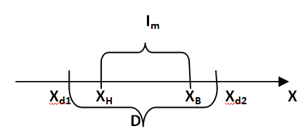
относительного расположения. Рассмотрим
рисунок 1.

1
вариант. Когда доверительный интервал
в области допустимых значений. При таком
расположении доверительный интервал
– часть области D
(внутри нее), поэтому вероятность
принадлежности результатов измерений
области D
больше доверительной вероятности
заданной. Вывод: Р≥
Р_d_З;
безопасность допустимая с вероятностью
более Р_d_З.

2
вариант.

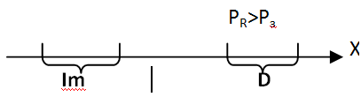
Рассуждая
также как и в 1 случае, вывод: что
безопасность недопустимая с вероятностью
более с Р_d_З.

3
вариант.

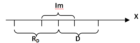
Этот
вариант возникает если одна из границ
попадает внутрь доверительного интервала.
Вывод: вероятность принадлежности
результатов измерения меньше P_з,как
в области допустимых значений так и в
области риска. Такой случай недопустимый,
т.к. не выполняется требования достижения
заданной вероятности.

6.Обеспечение
безопасности на предприятиях. Оценка
проводится по допустимым нормам
безопасности. Оценивается расположение
измеренного значения Х_м
по отношению к области D,
ошибка измерения учитывается системным
подходом, как к самому процессу измерения,
так и к контролю результатов измерения.
Допускаются к процессу измерения только
люди прошедшие специальное обучение и
имеющие свидетельство об этом. Организация,
которая занимается измерением, должна
иметь лицензию на этот вид деятельности
и измерения производить только по
утвержденным методикам. Используют
приборы и оборудование только указанное
в этих методиках, приборы должны проходить
периодическую поверку в организациях
имеющих соответствующую лицензию, и
иметь отметку о пройденной поверке с
указанием даты. Все документы и результаты
измерений проверяются контролирующими
органами. Такой системный подход
позволяет знать ошибку допускаемую при
измерении, заранее она заложена в
методику измерения. Нормы допустимой
безопасности устанавливаются с учетом
этой ошибки, что в целом позволяет при
оценке не учитывать ошибку измерений.
Процедура измерений и оценка безопасности
существенно упрощается. Последнее
обстоятельство на предприятии очень
важно, поскольку оценке безопасности
принадлежит каждое рабочее место по
всем параметрам влияющих на безопасность.
Оценка безопасности на производстве
требует очень большого количества
измерений, которые необходимо повторять.
Каждый руководитель подразделения
несет ответственность за своих
подчиненных. .Работа включает обучение
и проверку знаний техники безопасности.
2. Необходимо вести контроль систем и
оборудования обеспечивающих безопасность
на рабочих местах. 3. Необходимо проводить
планирование ремонтных работ по
ликвидации опасных воздействий. 4. Каждый
руководитель обязан иметь документацию
по обследованию рабочих мест и
самостоятельно оценивать безопасность.
5. Помощь оказывает специальные
подразделения или ответственные лица
в зависимости от размера предприятия.
1. Отдел техники безопасности: вопросы
производственной безопасности. 2.
Экологический отдел: занимается вопросами
экологической безопасности. 3. Штаб
гражданской обороны: безопасность на
случай ЧС.

7.
Понятие
о вредных веществах. По
отношению к человеку или другому объекту,
любое вещество может быть вредным,
нейтральным или полезным. Вредные
вещества – это такие вещества, которые
при контакте с организмом человека
могут вызывать производственные травмы,
профессиональные заболевания или
отклонения в состоянии здоровья,
обнаруживаемые современными методами
как в процессе работы, так и в отдаленные
сроки жизни настоящего и последующего
поколений. Из определения следует, что
вредные вещества могут воздействовать
на внутренние органы человека, а также
оказывать внешнее воздействие, опасность
которого, прежде всего в нанесении
травмы, среди вредных веществ отдельную
группу составляют вещества, которые
при попадании в живой организм вызывают
отравление. Наука изучающая отравления
называется токсикология, а такое
воздействие токсичным. Отравление –
это явные и достаточно стойкие нарушения
функций организма вызванные химическими
веществами, особый класс составляет
яды, яды – это токсичные вещества
вызывающие отравления в сравнительно
малых дозах. Воздействие вредных веществ
на организм человека в токсикологии
рассматривается в зависимости от пути
проникновения этих веществ в организм.
Выделяется 4 основных пути проникновения:
1. Через органы дыхания. 2. Желудочно-кишечный
тракт. 3. Кожа. 4. Слизистую оболочку глаз.
Понятие
о токсичном воздействии вредных веществ
на организм человека.

Среди
вредных веществ отдельную группу
составляют вещества, которые при
попадании в живой организм вызывают
отравление. Наука изучающая отравления
называется токсикология, а такое
воздействие токсичным. Отравление –
это явные и достаточно стойкие нарушения
функций организма вызванные химическими
веществами, особый класс составляет
яды, яды – это токсичные вещества
вызывающие отравления в сравнительно
малых дозах. Воздействие вредных веществ
на организм человека в токсикологии
рассматривается в зависимости от пути
проникновения этих веществ в организм.
Выделяется 4 основных пути проникновения:
1. Через органы дыхания. 2. Желудочно-кишечный
тракт. 3. Кожа. 4. Слизистую оболочку глаз.
Процессы эти сложные. Токсические
вещества в организме распределяются
не одинаково. Некоторые из них способны
к накоплению в определенных тканях.
Свинец накапливается в основном в
костях, марганец в печени, ртуть в почках
и толстой кишке, выделение токсичных
веществ из организма происходит тем же
путем, что и поступление. Не прореагировавшие
пары или газы частично или полностью
удаляются через легкие. Значительное
количество токсических веществ и
продуктов их превращения выделяется
через почки и кожные покровы, в последнем
случае процесс в основном совершают
сальные и потовые железы. Выделение
некоторых токсических веществ в составе
женского молока, это свинец, ртуть,
алкоголь. Это создает опасность отравления
грудных детей. Беременных женщин и
кормящих матерей следует временно
отстранить от производственных операций,
выделяющих токсические вещества.
Токсическое действие вредных веществ
может способствовать общему ослаблению
организма, в частности снижению
сопротивляемости к инфекции, например
известны зависимость между развитием
гриппа, ангины, пневмонии и наличием в
организме таких веществ как свинец,
сероводород, бензол.

Соседние файлы в предмете [НЕСОРТИРОВАННОЕ]

Источник

Константин Кравчик доходчиво объясняет, что такое доверительный интервал в медицинских исследованиях и как его использовать

«Катрен-Стиль» продолжает публикацию цикла Константина Кравчика о медицинской статистике. В двух предыдущих статьях автор касался объяснения таких понятий, как размер выборки, генеральная совокупность, статистическая гипотеза и классификацию шкал.

фото_Константин-Кравчик.png""

Досье КС

Константин Кравчик

Математик-аналитик. Специалист в области статистических исследований в медицине и гуманитарных науках

Город: Москва

Очень часто в статьях по клиническим исследованиям можно встретить загадочное словосочетание: «доверительный интервал» (95 % ДИ или 95 % CI — confidence interval). Например, в статье может быть написано: «Для оценки значимости различий использовали t-критерий Стьюдента с расчетом 95 % доверительного интервала».

Какого же значение «95 % доверительного интервала» и зачем его рассчитывать?

Что такое доверительный интервал? — Это диапазон, в котором находятся истинные средние значения в генеральной совокупности. А что, бывают «неистинные» средние значения? В каком‑то смысле да, бывают. В прошлой статье мы объясняли, что невозможно измерить интересующий параметр во всей генеральной совокупности, поэтому исследователи довольствуются ограниченной выборкой. В этой выборке (например, по массе тела) есть одно среднее значение (определенный вес), по которому мы и судим о среднем значении во всей генеральной совокупности. Однако едва ли средний вес в выборке (особенно небольшой) совпадет со средним весом в генеральной совокупности. Поэтому более правильно рассчитывать и пользоваться диапазоном средних значений генеральной совокупности.

Например, представим, что 95 % доверительный интервал (95 % ДИ) по гемоглобину составляет от 110 до 122 г/л. Это означает, что с вероятностью 95 % истинное среднее значение по гемоглобину в генеральной совокупности будет находиться в пределах от 110 до 122 г/л. Иными словами, мы не знаем средний показатель гемоглобина в генеральной совокупности, но можем с 95 %-й вероятностью указать диапазон значений для этого признака.

Доверительный интервал особенно уместен для разницы в средних значениях между группами или, как это называют, в размере эффекта.

Допустим, мы сравнивали эффективность двух препаратов железа: давно присутствующего на рынке и только что зарегистрированного. После курса терапии оценили концентрацию гемоглобина в исследуемых группах пациентов, и статистическая программа нам посчитала, что разность между средними значениями двух групп с вероятностью 95 % находится в диапазоне от 1,72 до 14,36 г/л (табл. 1).

Табл. 1. Критерий для независимых выборок
(сравниваются группы по уровню гемоглобина)

t-критерий	Значимость (2-сторонняя)	Разность средних	95 % доверительный интервал для разности
	Нижняя	Верхняя
2,609	0,014	8,048	1,7274	14,3678

Трактовать это следует так: у части пациентов генеральной совокупности, которая принимает новый препарат, гемоглобин будет выше в среднем на 1,72–14,36 г/л, чем у тех, кто принимал уже известный препарат.

Иными словами, в генеральной совокупности разность в средних значениях по гемоглобину у групп с 95 %-й вероятностью находится в этих пределах. Судить, много это или мало, будет уже исследователь. Смысл всего этого в том, что мы работаем не с одним средним значением, а с диапазоном значений, следовательно, мы более достоверно оцениваем разницу по параметру между группами.

В статистических пакетах, на усмотрение исследователя, можно самостоятельно сужать или расширять границы доверительного интервала. Снижая вероятности доверительного интервала, мы сужаем диапазон средних. Например, при 90 % ДИ диапазон средних (или разницы средних) будет уже, чем при 95 %.

И наоборот, увеличение вероятности до 99 % расширяет диапазон значений. При сравнении групп нижняя граница ДИ может пересечь нулевую отметку. Например, если мы расширили границы доверительного интервала до 99 %, то границы интервала расположились от –1 до 16 г/л. Это означает, что в генеральной совокупности есть группы, различие средних между которыми по изучаемому признаку равняется 0 (М=0).

При помощи доверительного интервала можно проверять статистические гипотезы. Если доверительный интервал пересекает нулевое значение, то нулевая гипотеза, предполагающая, что группы не различаются по изучаемому параметру, верна. Пример описан выше, когда мы расширили границы до 99 %. Где‑то в генеральной совокупности у нас нашлись группы, которые никак не различались.

Почему рекомендуется смотреть на доверительный интервал? Для большей наглядности обратимся к рисунку.

95% доверительный интервал разницы по гемоглобину, (г/л)

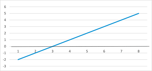
95% доверительный интервал разницы по гемоглобину, (г/л).png

На рисунке в виде линии изображен 95 % доверительный интервал разницы средних значений по гемоглобину между двумя группами. Линия проходит нулевую отметку, следовательно, имеет место разница между средними значениями, равная нулю, что подтверждает нулевую гипотезу о том, что группы не различаются. Диапазон разницы между группами лежит от –2 до 5 г/л, Это означает, что гемоглобин может как снизиться на 2 г/л, так и повыситься на 5 г/л.

Доверительный интервал — очень важный показатель. Благодаря ему можно посмотреть, были ли различия в группах действительно за счет разности средних или за счет большой выборки, т. к. при большой выборке шансы найти различия больше, чем при малой.

На практике это может выглядеть так. Мы взяли выборку в 1000 человек, измерили уровень гемоглобина и обнаружили, что доверительный интервал разницы средних лежит от 1,2 до 1,5 г/л. Уровень статистической значимости при этом p<0,05.

Мы видим, что концентрация гемоглобина повысилась, но практически незаметно, следовательно, статистическая значимость появилась именно за счет объема выборки.

Доверительный интервал может быть высчитан не только для средних значений, но и для пропорций (и отношений рисков). Например, нас интересует доверительный интервал пропорций пациентов, которые достигли ремиссии, принимая разработанное лекарство. Допустим, что 95 % ДИ для пропорций, т. е. для доли таких пациентов, лежит в пределах 0,60–0,80. Таким образом, мы можем сказать, что наше лекарство оказывает терапевтический эффект от 60 до 80 % случаев.

Источник

Быстро понять понимание 95% доверительного интервала в одной статье

Всесторонне знать ответы главных богов и сетевые данные, чтобы понять 95% доверительный интервал этой статьи.

Сделайте вывод первым

Наиболее часто встречающаяся пара доверительных интерваловошибкапонимание:

В пределах 95% доверительного интервала существует 95% вероятность того, что истинные параметры включены (ошибка !!!)

Модель, построенная с доверительной зоной 95%, означает, что параметры модели с вероятностью 95% являются оценкой истинного значения функции, которую пытаются аппроксимировать (ошибка !!!)

верныйОбъяснение должно быть таким:

Доверительный интервал 95% означает, что если вы выполните те же действия для выбора образцов и расчета доверительного интервала,Тогда при 100-кратном таком независимом процессе существует 95% вероятность того, что рассчитанный вами интервал будет содержать истинное значение параметра, то есть будет около 95 доверительных интервалов, которые будут содержать истинное значение.

И для определенного расчетаМы не можем обсуждать вероятность того, что определенный доверительный интервал содержит истинное значение.

Частота школы (частотный) 95% доверительный интервал, который мы обычно используем, не означает, что вероятность того, что истинное значение находится в пределах этого интервала, составляет 95%. Значение истины либо присутствует, либо нет. из-заВ частотной школе значение истинности является константой, а не случайной величиной (последняя — байесовская школа). , Поэтому мы не описываем вероятность истинности значения. В этом вопросе ключ к пониманию состоит в том, что мыВероятностное описание этого метода построения доверительного интервала, Ни истинное значение, ни интервал, который мы рассчитали.

Другими словами, мы можем сказать,Если мы повторим выборку и воспользуемся этим методом для построения доверительного интервала после каждой выборки, 95% доверительного интервала будет содержать истинное значение.. Однако (в частотной школе) мыНевозможно обсуждать вероятность того, что один из доверительных интервалов содержит истинное значение.

Ссылка из: Как понять 95% доверительный интервал? -Ответ Гуань Чжиюаня-Зная https://www.zhihu.com/question/26419030/answer/70589735

Детальный анализ

Ссылка на снимок экрана: Zhihu-Как понять 95% доверительный интервал?

-Ответ студентки Ма-Почти знаюhttps://www.zhihu.com/question/26419030/answer/274472266
Авторские права принадлежат автору

Предполагается, что он будет разделен на «Точечная оценка«с участием»Оценка интервала”

Интервальная оценка также называетсяОценка доверительного интервала, Для получения доверительного интервала требуется выборочная статистика (например, среднее значение) и вычисление дисперсии по данным. Центральная предельная теорема говорит нам, что среднее значение будет близко к распределению Гаусса. Мы можем использовать стандартное отклонение для вычисления вероятности что истинное ожидание попадает в выбранный интервал. Например, область с вероятностью 0,95 с центром на среднем значении μ ^ равна (на основе распределения Гаусса):

Отступление: в экспериментах с машинным обучением мы обычно используем среднюю ошибку выборок тестового набора для оценки ошибки обобщения. Обычно мы говорим, что алгоритм A лучше, чем алгоритм B, что означает, что верхняя граница 95% доверительного интервала ошибка алгоритма A меньше, чем у алгоритма. Нижняя граница 95% доверительного интервала для ошибки A.

В заключении

Перевод из блога научной сети Ди Юэбао
Адрес ссылки:http://blog.sciencenet.cn/blog-925634-870778.html

Предполагая, что теперь он находится на уровне достоверности 95% (95% также называют уровнем достоверности, что является привычкой в статистике и может корректироваться в зависимости от приложения.），95% доверительный интервал может быть получен для каждой выборки, взятой из совокупности, и доверительный интервал, полученный для разных выборок, отличается, но по мере увеличения количества взятых выборок, например, отбирается 100 выборок и получается 100 выборок, Каждая выборка соответствует доверительному интервалу, поэтому 95 из 100 доверительных интервалов, полученных из 100 выборок, содержат истинное среднее значение генеральной совокупности.

Доверительный интервал будет варьироваться от образца к образцу (Как рассчитывается доверительный интервал? Черезобразец(Образец) рассчитано), и не все интервалы содержат значения истинности,Интервал подобен забросу сети для захвата общих неизвестных параметров. Не все места, где используется сеть, могут захватывать общие параметры, которые мы хотим.

Источник

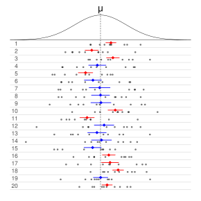
Each row of points is a sample from the same normal distribution. The colored lines are 50% confidence intervals for the mean, μ. At the center of each interval is the sample mean, marked with a diamond. The blue intervals contain the population mean, and the red ones do not.

In frequentist statistics, a confidence interval (CI) is a range of estimates for an unknown parameter. A confidence interval is computed at a designated confidence level; the 95% confidence level is most common, but other levels, such as 90% or 99%, are sometimes used.^[1]^[2] The confidence level represents the long-run proportion of CIs (at the given confidence level) that theoretically contain the true value of the parameter. For example, out of all intervals computed at the 95% level, 95% of them should contain the parameter’s true value.^[3]

Factors affecting the width of the CI include the sample size, the variability in the sample, and the confidence level.^[4] All else being the same, a larger sample produces a narrower confidence interval, greater variability in the sample produces a wider confidence interval, and a higher confidence level produces a wider confidence interval.^[5]

Definition[edit]

Let X be a random sample from a probability distribution with statistical parameter θ, which is a quantity to be estimated, and φ, representing quantities that are not of immediate interest. A confidence interval for the parameter θ, with confidence level or coefficient γ, is an interval ${displaystyle ( u(X),v(X) ) }$ determined by random variables ${displaystyle u(X) }$ and ${displaystyle v(X) }$ with the property:

${displaystyle Pr{ u(X)<theta <v(X) } = gamma quad {text{ for every }}(theta ,varphi )~.}$

The number γ, whose typical value is close to but not greater than 1, is sometimes given in the form ${displaystyle 1-alpha }$ (or as a percentage ${displaystyle 100%cdot (1-alpha ) }$ ), where ${displaystyle alpha }$ is a small positive number, often 0.05 .

It is important for the bounds ${displaystyle u(X) }$ and ${displaystyle v(X) }$ to be specified in such a way that as long as X is collected randomly, every time we compute a confidence interval, there is probability γ that it would contain θ, the true value of the parameter being estimated. This should hold true for any actual θ and φ.^[2]

Approximate confidence intervals[edit]

In many applications, confidence intervals that have exactly the required confidence level are hard to construct, but approximate intervals can be computed. The rule for constructing the interval may be accepted as providing a confidence interval at level $gamma$ if

${displaystyle Pr{ u(X)<theta <v(X) } approx gamma quad {text{ for every }}(theta ,varphi )}$

to an acceptable level of approximation. Alternatively, some authors^[6] simply require that

${displaystyle Pr{ u(X)<theta <v(X) } geq gamma quad {text{ for every }}(theta ,varphi )~,}$

which is useful if the probabilities are only partially identified or imprecise, and also when dealing with discrete distributions. Confidence limits of form

${displaystyle Pr{ u(X)<theta } geq gamma ~}$ and ${displaystyle Pr{ theta <v(X) }geq gamma ~}$

are called conservative;^[7]^(p 210) accordingly, one speaks of conservative confidence intervals and, in general, regions.

Desired properties[edit]

When applying standard statistical procedures, there will often be standard ways of constructing confidence intervals. These will have been devised so as to meet certain desirable properties, which will hold given that the assumptions on which the procedure relies are true. These desirable properties may be described as: validity, optimality, and invariance.

Of the three, «validity» is most important, followed closely by «optimality». «Invariance» may be considered as a property of the method of derivation of a confidence interval, rather than of the rule for constructing the interval. In non-standard applications, these same desirable properties would be sought:

Validity[edit]

This means that the nominal coverage probability (confidence level) of the confidence interval should hold, either exactly or to a good approximation.

Optimality[edit]

This means that the rule for constructing the confidence interval should make as much use of the information in the data-set as possible.

Recall that one could throw away half of a dataset and still be able to derive a valid confidence interval. One way of assessing optimality is by the length of the interval so that a rule for constructing a confidence interval is judged better than another if it leads to intervals whose lengths are typically shorter.

Invariance[edit]

In many applications, the quantity being estimated might not be tightly defined as such.

For example, a survey might result in an estimate of the median income in a population, but it might equally be considered as providing an estimate of the logarithm of the median income, given that this is a common scale for presenting graphical results. It would be desirable that the method used for constructing a confidence interval for the median income would give equivalent results when applied to constructing a confidence interval for the logarithm of the median income: Specifically the values at the ends of the latter interval would be the logarithms of the values at the ends of former interval.

Methods of derivation[edit]

For non-standard applications, there are several routes that might be taken to derive a rule for the construction of confidence intervals. Established rules for standard procedures might be justified or explained via several of these routes. Typically a rule for constructing confidence intervals is closely tied to a particular way of finding a point estimate of the quantity being considered.

Summary statistics[edit]

This is closely related to the method of moments for estimation. A simple example arises where the quantity to be estimated is the population mean, in which case a natural estimate is the sample mean. Similarly, the sample variance can be used to estimate the population variance. A confidence interval for the true mean can be constructed centered on the sample mean with a width which is a multiple of the square root of the sample variance.

Likelihood theory[edit]

Estimates can be constructed using the maximum likelihood principle, the likelihood theory for this provides two ways of constructing confidence intervals or confidence regions for the estimates.

Estimating equations[edit]

The estimation approach here can be considered as both a generalization of the method of moments and a generalization of the maximum likelihood approach. There are corresponding generalizations of the results of maximum likelihood theory that allow confidence intervals to be constructed based on estimates derived from estimating equations.^{[citation needed]}

Hypothesis testing[edit]

If hypothesis tests are available for general values of a parameter, then confidence intervals/regions can be constructed by including in the 100 p % confidence region all those points for which the hypothesis test of the null hypothesis that the true value is the given value is not rejected at a significance level of (1 − p) .^[7]^{(§ 7.2 (iii))}

Bootstrapping[edit]

In situations where the distributional assumptions for the above methods are uncertain or violated, resampling methods allow construction of confidence intervals or prediction intervals. The observed data distribution and the internal correlations are used as the surrogate for the correlations in the wider population.

Central limit theorem[edit]

The central limit theorem is a refinement of the law of large numbers. For a large number of independent identically distributed random variables ${displaystyle X_{1},...,X_{n} ,}$ with finite variance, the average ${displaystyle {overline {X}}_{n} }$ approximately has a normal distribution, no matter what the distribution of the ${displaystyle X_{i} }$ is, with the approximation roughly improving in proportion to ${displaystyle {sqrt {n }}.}$ ^[2]

Example[edit]

Suppose {X₁, …, X_n} is an independent sample from a normally distributed population with unknown parameters mean μ and variance σ². Let

${bar {X}}=(X_{1}+cdots +X_{n})/n,,$

${displaystyle S^{2}={frac {1}{n-1}}sum _{i=1}^{n}(X_{i}-{bar {X}},)^{2}.}$

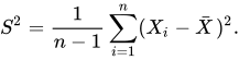
Where X is the sample mean, and S² is the sample variance. Then

$T={frac {{bar {X}}-mu }{S/{sqrt {n}}}}$

has a Student’s t distribution with n − 1 degrees of freedom.^[8] Note that the distribution of T does not depend on the values of the unobservable parameters μ and σ²; i.e., it is a pivotal quantity. Suppose we wanted to calculate a 95% confidence interval for μ. Then, denoting c as the 97.5th percentile of this distribution,

${displaystyle Pr(-cleq Tleq c)=0.95}$

Note that «97.5th» and «0.95» are correct in the preceding expressions. There is a 2.5% chance that $T$ will be less than $-c$ and a 2.5% chance that it will be larger than ${displaystyle +c}$ . Thus, the probability that $T$ will be between $-c$ and ${displaystyle +c}$ is 95%.

Consequently,

$Pr left({bar {X}}-{frac {cS}{sqrt {n}}}leq mu leq {bar {X}}+{frac {cS}{sqrt {n}}}right)=0.95,$

and we have a theoretical (stochastic) 95% confidence interval for μ.

After observing the sample we find values x for X and s for S, from which we compute the confidence interval

${displaystyle left[{bar {x}}-{frac {cs}{sqrt {n}}},{bar {x}}+{frac {cs}{sqrt {n}}}right].}$

In this bar chart, the top ends of the brown bars indicate observed means and the red line segments («error bars») represent the confidence intervals around them. Although the error bars are shown as symmetric around the means, that is not always the case. In most graphs, the error bars do not represent confidence intervals (e.g., they often represent standard errors or standard deviations)

Interpretation[edit]

Various interpretations of a confidence interval can be given (taking the 95% confidence interval as an example in the following).

The confidence interval can be expressed in terms of a long-run frequency in repeated samples (or in resampling): «Were this procedure to be repeated on numerous samples, the proportion of calculated 95% confidence intervals that encompassed the true value of the population parameter would tend toward 95%.»^[9]
The confidence interval can be expressed in terms of probability with respect to a single theoretical (yet to be realized) sample: «There is a 95% probability that the 95% confidence interval calculated from a given future sample will cover the true value of the population parameter.» ^[10] This essentially reframes the «repeated samples» interpretation as a probability rather than a frequency. See Neyman construction.
The confidence interval can be expressed in terms of statistical significance, e.g.: «The 95% confidence interval represents values that are not statistically significantly different from the point estimate at the .05 level«.^[11]

Interpretation of the 95% confidence interval in terms of statistical significance.

Common misunderstandings[edit]

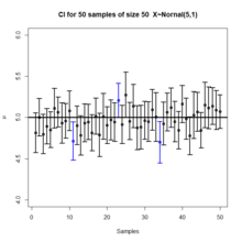
Plot of 50 confidence intervals from 50 samples generated from a normal distribution.

Counterexamples[edit]

Since confidence interval theory was proposed, a number of counter-examples to the theory have been developed to show how the interpretation of confidence intervals can be problematic, at least if one interprets them naïvely.

Confidence procedure for uniform location[edit]

Welch^[21] presented an example which clearly shows the difference between the theory of confidence intervals and other theories of interval estimation (including Fisher’s fiducial intervals and objective Bayesian intervals). Robinson^[22] called this example «[p]ossibly the best known counterexample for Neyman’s version of confidence interval theory.» To Welch, it showed the superiority of confidence interval theory; to critics of the theory, it shows a deficiency. Here we present a simplified version.

Suppose that $X_{1},X_{2}$ are independent observations from a Uniform(θ − 1/2, θ + 1/2) distribution. Then the optimal 50% confidence procedure for $theta$ is^[23]

${displaystyle {bar {X}}pm {begin{cases}{dfrac {|X_{1}-X_{2}|}{2}}&{text{if }}|X_{1}-X_{2}|<1/2\[8pt]{dfrac {1-|X_{1}-X_{2}|}{2}}&{text{if }}|X_{1}-X_{2}|geq 1/2.end{cases}}}$

A fiducial or objective Bayesian argument can be used to derive the interval estimate

${displaystyle {bar {X}}pm {frac {1-|X_{1}-X_{2}|}{4}},}$

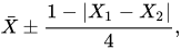
which is also a 50% confidence procedure. Welch showed that the first confidence procedure dominates the second, according to desiderata from confidence interval theory; for every ${displaystyle theta _{1}neq theta }$ , the probability that the first procedure contains $theta _{1}$ is less than or equal to the probability that the second procedure contains $theta _{1}$ . The average width of the intervals from the first procedure is less than that of the second. Hence, the first procedure is preferred under classical confidence interval theory.

However, when ${displaystyle |X_{1}-X_{2}|geq 1/2}$ , intervals from the first procedure are guaranteed to contain the true value $theta$ : Therefore, the nominal 50% confidence coefficient is unrelated to the uncertainty we should have that a specific interval contains the true value. The second procedure does not have this property.

Moreover, when the first procedure generates a very short interval, this indicates that $X_{1},X_{2}$ are very close together and hence only offer the information in a single data point. Yet the first interval will exclude almost all reasonable values of the parameter due to its short width. The second procedure does not have this property.

The two counter-intuitive properties of the first procedure—100% coverage when $X_{1},X_{2}$ are far apart and almost 0% coverage when $X_{1},X_{2}$ are close together—balance out to yield 50% coverage on average. However, despite the first procedure being optimal, its intervals offer neither an assessment of the precision of the estimate nor an assessment of the uncertainty one should have that the interval contains the true value.

This counter-example is used to argue against naïve interpretations of confidence intervals. If a confidence procedure is asserted to have properties beyond that of the nominal coverage (such as relation to precision, or a relationship with Bayesian inference), those properties must be proved; they do not follow from the fact that a procedure is a confidence procedure.

Confidence procedure for ω²[edit]

Steiger^[24] suggested a number of confidence procedures for common effect size measures in ANOVA. 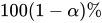Morey et al.^[18] point out that several of these confidence procedures, including the one for ω², have the property that as the F statistic becomes increasingly small—indicating misfit with all possible values of ω²—the confidence interval shrinks and can even contain only the single value ω² = 0; that is, the CI is infinitesimally narrow (this occurs when ${displaystyle pgeq 1-alpha /2}$ for a $100(1-alpha)%$ CI).

This behavior is consistent with the relationship between the confidence procedure and significance testing: as F becomes so small that the group means are much closer together than we would expect by chance, a significance test might indicate rejection for most or all values of ω². Hence the interval will be very narrow or even empty (or, by a convention suggested by Steiger, containing only 0). However, this does not indicate that the estimate of ω² is very precise. In a sense, it indicates the opposite: that the trustworthiness of the results themselves may be in doubt. This is contrary to the common interpretation of confidence intervals that they reveal the precision of the estimate.

History[edit]

Confidence intervals were introduced by Jerzy Neyman in 1937.^[25] Statisticians quickly took to the idea, but adoption by scientists was more gradual. Some authors in medical journals promoted confidence intervals as early as the 1970s. Despite this, confidence intervals were rarely used until the following decade, when they quickly became standard.^[26] By the late 1980s, medical journals began to require the reporting of confidence intervals.^[27]

References[edit]

^ Zar, Jerrold H. (199). Biostatistical Analysis (4th ed.). Upper Saddle River, N.J.: Prentice Hall. pp. 43–45. ISBN 978-0130815422. OCLC 39498633.
^ ^a ^b ^c Dekking, Frederik Michel; Kraaikamp, Cornelis; Lopuhaä, Hendrik Paul; Meester, Ludolf Erwin (2005). «A Modern Introduction to Probability and Statistics». Springer Texts in Statistics. doi:10.1007/1-84628-168-7. ISBN 978-1-85233-896-1. ISSN 1431-875X.
^ Illowsky, Barbara. Introductory statistics. Dean, Susan L., 1945-, Illowsky, Barbara., OpenStax College. Houston, Texas. ISBN 978-1-947172-05-0. OCLC 899241574.
^ Hazra, Avijit (October 2017). «Using the confidence interval confidently». Journal of Thoracic Disease. 9 (10): 4125–4130. doi:10.21037/jtd.2017.09.14. ISSN 2072-1439. PMC 5723800. PMID 29268424.
^ Khare, Vikas; Nema, Savita; Baredar, Prashant (2020). Ocean Energy Modeling and Simulation with Big Data Computational Intelligence for System Optimization and Grid Integration. ISBN 978-0-12-818905-4. OCLC 1153294021.
^ Roussas, George G. (1997). A Course in Mathematical Statistics (2nd ed.). Academic Press. p. 397.
^ ^a ^b Cox, D.R.; Hinkley, D.V. (1974). Theoretical Statistics. Chapman & Hall.
^ Rees. D.G. (2001) Essential Statistics, 4th Edition, Chapman and Hall/CRC. ISBN 1-58488-007-4 (Section 9.5)
^ Cox D.R., Hinkley D.V. (1974) Theoretical Statistics, Chapman & Hall, p49, p209
^ ^a ^b Neyman, J. (1937). «Outline of a Theory of Statistical Estimation Based on the Classical Theory of Probability». Philosophical Transactions of the Royal Society A. 236 (767): 333–380. Bibcode:1937RSPTA.236..333N. doi:10.1098/rsta.1937.0005. JSTOR 91337.
^ Cox D.R., Hinkley D.V. (1974) Theoretical Statistics, Chapman & Hall, pp 214, 225, 233
^ Kalinowski, Pawel (2010). «Identifying Misconceptions about Confidence Intervals» (PDF). Retrieved 2021-12-22.
^ «Archived copy» (PDF). Archived from the original (PDF) on 2016-03-04. Retrieved 2014-09-16.{{cite web}}: CS1 maint: archived copy as title (link)
^ Hoekstra, R., R. D. Morey, J. N. Rouder, and E-J. Wagenmakers, 2014. Robust misinterpretation of confidence intervals. Psychonomic Bulletin Review, in press. [1]
^ Scientists’ grasp of confidence intervals doesn’t inspire confidence, Science News, July 3, 2014
^ ^a ^b Greenland, Sander; Senn, Stephen J.; Rothman, Kenneth J.; Carlin, John B.; Poole, Charles; Goodman, Steven N.; Altman, Douglas G. (April 2016). «Statistical tests, P values, confidence intervals, and power: a guide to misinterpretations». European Journal of Epidemiology. 31 (4): 337–350. doi:10.1007/s10654-016-0149-3. ISSN 0393-2990. PMC 4877414. PMID 27209009.
^ Helske, Jouni; Helske, Satu; Cooper, Matthew; Ynnerman, Anders; Besancon, Lonni (2021-08-01). «Can Visualization Alleviate Dichotomous Thinking? Effects of Visual Representations on the Cliff Effect». IEEE Transactions on Visualization and Computer Graphics. Institute of Electrical and Electronics Engineers (IEEE). 27 (8): 3397–3409. arXiv:2002.07671. doi:10.1109/tvcg.2021.3073466. ISSN 1077-2626. PMID 33856998. S2CID 233230810.
^ ^a ^b Morey, R. D.; Hoekstra, R.; Rouder, J. N.; Lee, M. D.; Wagenmakers, E.-J. (2016). «The Fallacy of Placing Confidence in Confidence Intervals». Psychonomic Bulletin & Review. 23 (1): 103–123. doi:10.3758/s13423-015-0947-8. PMC 4742505. PMID 26450628.
^ «1.3.5.2. Confidence Limits for the Mean». nist.gov. Archived from the original on 2008-02-05. Retrieved 2014-09-16.
^ Mayo, D. G. (1981) «In defence of the Neyman–Pearson theory of confidence intervals», Philosophy of Science, 48 (2), 269–280. JSTOR 187185
^ Welch, B. L. (1939). «On Confidence Limits and Sufficiency, with Particular Reference to Parameters of Location». The Annals of Mathematical Statistics. 10 (1): 58–69. doi:10.1214/aoms/1177732246. JSTOR 2235987.
^ Robinson, G. K. (1975). «Some Counterexamples to the Theory of Confidence Intervals». Biometrika. 62 (1): 155–161. doi:10.2307/2334498. JSTOR 2334498.
^ Pratt, J. W. (1961). «Book Review: Testing Statistical Hypotheses. by E. L. Lehmann». Journal of the American Statistical Association. 56 (293): 163–167. doi:10.1080/01621459.1961.10482103. JSTOR 2282344.
^ Steiger, J. H. (2004). «Beyond the F test: Effect size confidence intervals and tests of close fit in the analysis of variance and contrast analysis». Psychological Methods. 9 (2): 164–182. doi:10.1037/1082-989x.9.2.164. PMID 15137887.
^ [Neyman, J., 1937. Outline of a theory of statistical estimation based on the classical theory of probability. Philosophical Transactions of the Royal Society of London. Series A, Mathematical and Physical Sciences, 236(767), pp.333-380]
^ Altman, Douglas G. (1991). «Statistics in medical journals: Developments in the 1980s». Statistics in Medicine. 10 (12): 1897–1913. doi:10.1002/sim.4780101206. ISSN 1097-0258. PMID 1805317.
^ Sandercock, Peter A.G. (2015). «Short History of Confidence Intervals». Stroke. Ovid Technologies (Wolters Kluwer Health). 46 (8): e184-7. doi:10.1161/strokeaha.115.007750. ISSN 0039-2499. PMID 26106115.

Bibliography[edit]

Fisher, R.A. (1956) Statistical Methods and Scientific Inference. Oliver and Boyd, Edinburgh. (See p. 32.)
Freund, J.E. (1962) Mathematical Statistics Prentice Hall, Englewood Cliffs, NJ. (See pp. 227–228.)
Hacking, I. (1965) Logic of Statistical Inference. Cambridge University Press, Cambridge. ISBN 0-521-05165-7
Keeping, E.S. (1962) Introduction to Statistical Inference. D. Van Nostrand, Princeton, NJ.
Kiefer, J. (1977). «Conditional Confidence Statements and Confidence Estimators (with discussion)». Journal of the American Statistical Association. 72 (360a): 789–827. doi:10.1080/01621459.1977.10479956. JSTOR 2286460.
Mayo, D. G. (1981) «In defence of the Neyman–Pearson theory of confidence intervals», Philosophy of Science, 48 (2), 269–280. JSTOR 187185
Neyman, J. (1937) «Outline of a Theory of Statistical Estimation Based on the Classical Theory of Probability» Philosophical Transactions of the Royal Society of London A, 236, 333–380. (Seminal work.)
Robinson, G.K. (1975). «Some Counterexamples to the Theory of Confidence Intervals». Biometrika. 62 (1): 155–161. doi:10.1093/biomet/62.1.155. JSTOR 2334498.
Savage, L. J. (1962), The Foundations of Statistical Inference. Methuen, London.
Smithson, M. (2003) Confidence intervals. Quantitative Applications in the Social Sciences Series, No. 140. Belmont, CA: SAGE Publications. ISBN 978-0-7619-2499-9.

Mehta, S. (2014) Statistics Topics ISBN 978-1-4992-7353-3
«Confidence estimation», Encyclopedia of Mathematics, EMS Press, 2001 [1994]
Morey, R. D.; Hoekstra, R.; Rouder, J. N.; Lee, M. D.; Wagenmakers, E.-J. (2016). «The fallacy of placing confidence in confidence intervals». Psychonomic Bulletin & Review. 23 (1): 103–123. doi:10.3758/s13423-015-0947-8. PMC 4742505. PMID 26450628.

External links[edit]

The Exploratory Software for Confidence Intervals tutorial programs that run under Excel
Confidence interval calculators for R-Squares, Regression Coefficients, and Regression Intercepts
Weisstein, Eric W. «Confidence Interval». MathWorld.
CAUSEweb.org Many resources for teaching statistics including Confidence Intervals.
An interactive introduction to Confidence Intervals
Confidence Intervals: Confidence Level, Sample Size, and Margin of Error by Eric Schulz, the Wolfram Demonstrations Project.
Confidence Intervals in Public Health. Straightforward description with examples and what to do about small sample sizes or rates near 0.

Источник

Доверительная вероятность р 95 означает что риск допустить ошибку составляет не более

95% доверительный интервал разницы по гемоглобину, (г/л)

Быстро понять понимание 95% доверительного интервала в одной статье

Сделайте вывод первым

Детальный анализ

В заключении