Explanation
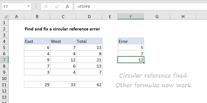
Circular reference errors occur when a formula refers back to its own cell. For example, in the example shown, the formula in F7 is:
=F5+F6+F7
This creates a circular reference because the formula, entered in cell F7, refers to F7. This in turn throws off other formula results in D7, C11, and D11:
=F7 // formula in C7
=SUM(B7:C7) // formula in D7
=SUM(C5:C9) // formula in C11
=SUM(D5:D9) // formula in D11
Circular references can cause many problems (and a lot of confusion) because they may cause other formulas to return zero, or a different incorrect result.
The circular reference error message
When a circular reference occurs in a spreadsheet, you’ll see a warning like this:
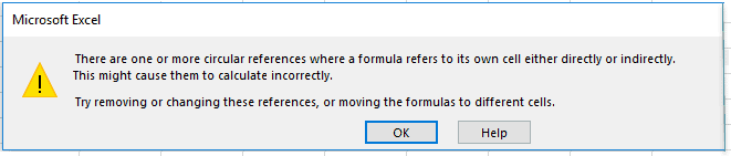
«There are one or more circular references where a formula refers to its own cell either directly or indirectly. This might cause them to calculate incorrectly. Try removing or changing these references, or moving the formulas to different cells.»

This warning will appear sporadically while editing, or when a worksheet is opened.
Finding and fixing circular references
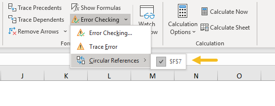
To resolve circular references, you’ll need to find the cell(s) with incorrect cell references and adjust as needed. However, unlike other errors (#N/A, #VALUE!, etc.) circular references don’t appear directly in the cell. To find the source of a circular reference error, use the Error Checking menu on the Formulas tab of the ribbon.

Select the Circular References item to see the source of circular references:
Below, the circular reference has been fixed and other formulas now return correct results:
Excel for Microsoft 365 Excel for Microsoft 365 for Mac Excel 2021 Excel 2021 for Mac Excel 2019 Excel 2019 for Mac Excel 2016 Excel 2016 for Mac Excel 2013 Excel 2010 Excel 2007 Excel for Mac 2011 Excel Starter 2010 More…Less
You’ve entered a formula, but it’s not working. Instead, you’ve got this message about a “circular reference.” Millions of people have the same problem, and it happens because your formula is trying to calculate itself, and you have a feature called iterative calculation turned off. Here’s what it looks like:
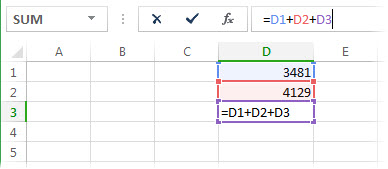
The formula =D1+D2+D3 breaks because it lives in cell D3, and it’s trying to calculate itself. To fix the problem, you can move the formula to another cell. Press Ctrl+X to cut the formula, select another cell, and press Ctrl+V to paste it.
Another common mistake is using a function that includes a reference to itself; for example, cell F3 contains =SUM(A3:F3). Here’s an example:

You can also try one of these techniques:
-
If you just entered a formula, start with that cell and check to see if you refer to the cell itself. For example, cell A3 might contain the formula =(A1+A2)/A3. Formulas like =A1+1 (in cell A1) also cause circular reference errors.
While you’re looking, check for indirect references. They happen when you put a formula in cell A1, and it uses another formula in B1 that in turn refers back to cell A1. If this confuses you, imagine what it does to Excel.
-
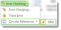
If you can’t find the error, click the Formulas tab, click the arrow next to Error Checking, point to Circular References, and then click the first cell listed in the submenu.
-
Review the formula in the cell. If you can’t determine whether the cell is the cause of the circular reference, click the next cell in the Circular References submenu.
-
Continue to review and correct the circular references in the workbook by repeating steps any or all of the steps 1 through 3 until the status bar no longer displays «Circular References.»
Tips
-
If you’re brand new to working with formulas, see Excel 2016 Essential Training at LinkedIn Learning.
-
The status bar in the lower-left corner displays Circular References and the cell address of one circular reference.
If you have circular references in other worksheets, but not in the active worksheet, the status bar displays only “Circular References” with no cell addresses.
-
You can move between cells in a circular reference by double-clicking the tracer arrow. The arrow indicates the cell that affects the value of the currently selected cell. You show the tracer arrow by clicking Formulas, and then click either Trace Precedents or Trace Dependents.
Learn about the circular reference warning message
The first time Excel finds a circular reference, it displays a warning message. Click OK or close the message window.
When you close the message, Excel displays either a zero or the last calculated value in the cell. And now you’re probably saying, «Hang on, a last calculated value?» Yes. In some cases, a formula can run successfully before it tries to calculate itself. For example, a formula that uses the IF function may work until a user enters an argument (a piece of data the formula needs to run properly) that causes the formula to calculate itself. When that happens, Excel retains the value from the last successful calculation.
If you suspect you have a circular reference in a cell that isn’t showing a zero, try this:
-
Click the formula in the formula bar, and then press Enter.
Important In many cases, if you create additional formulas that contain circular references, Excel won’t display the warning message again. The following list shows some, but not all, the scenarios in which the warning message will appear:
-
You create the first instance of a circular reference in any open workbook
-
You remove all circular references in all open workbooks, and then create a new circular reference
-
You close all workbooks, create a new workbook, and then enter a formula that contains a circular reference
-
You open a workbook that contains a circular reference
-
While no other workbooks are open, you open a workbook and then create a circular reference
Learn about iterative calculation
At times, you may want to use circular references because they cause your functions to iterate—repeat until a specific numeric condition is met. This can slow your computer down, so iterative calculations are usually turned off in Excel.
Unless you’re familiar with iterative calculations, you probably won’t want to keep any circular references intact. If you do, you can enable iterative calculations, but you need to determine how many times the formula should recalculate. When you turn on iterative calculations without changing the values for maximum iterations or maximum change, Excel stops calculating after 100 iterations, or after all values in the circular reference change by less than 0.001 between iterations, whichever comes first. However, you can control the maximum number of iterations and the amount of acceptable change.
-
Click File > Options > Formulas. If you’re using Excel for Mac, click the Excel menu, and then click Preferences > Calculation.
-
In the Calculation options section, select the Enable iterative calculation check box. On the Mac, click Use iterative calculation.
-
To set the maximum number of times that Excel will recalculate, type the number of iterations in the Maximum Iterations box. The higher the number of iterations, the more time that Excel needs to calculate a worksheet.
-
In the Maximum Change box, type the smallest value required for iteration to continue. This is the smallest change in any calculated value. The smaller the number, the more precise the result and the more time that Excel needs to calculate a worksheet.
An iterative calculation can have three outcomes:
-
The solution converges, which means a stable end result is reached. This is the desirable condition.
-
The solution diverges, which means that from iteration to iteration, the difference between the current and the previous result increases.
-
The solution switches between two values. For example, after the first iteration the result is 1, after the next iteration the result is 10, after the next iteration the result is 1, and so on.
Top of Page
Need more help?
You can always ask an expert in the Excel Tech Community or get support in the Answers community.

See also
Excel 2016 Essential Training
Overview of formulas in Excel
How to avoid broken formulas
Find and correct errors in formulas
Excel keyboard shortcuts and function keys
Excel functions (alphabetical)
Excel functions (by category)
Need more help?
A circular reference occurs when you end up having a formula in a cell – which in itself uses the cell reference (in which it’s been entered) for the calculation. If this statement seems a bit confusing, don’t worry by the end of this tutorial it will start to make sense.
In simple terms, a circular reference happens when a formula references back to its own cell directly or indirectly, creating an endless loop of calculations. This endless reference loop, if not stopped will keep changing the cell’s value every time.

For quick understanding, here’s an example.
In our example, there are a few numbers in column A and we are trying to calculate their sum using the SUM function in A7 cell. But inside the SUM function, we have passed the range as A1:A7.
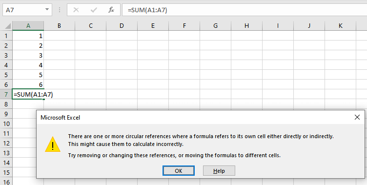
Since the supplied range also includes A7 cell (in which the result needs to be populated) so it creates an endless loop as Excel just keeps on adding the new value in cell A7, which keeps on incrementing.
This triggers Excel’s circular reference warning that says, «There are one or more circular references where a formula refers to its own cell either directly or indirectly. This might cause them to calculate incorrectly. Try removing or changing these references, or moving the formulas to different cells.».
Keep in mind that this is not an error since it will not stop further calculations or ask the user to change them. It is a warning that warns the user that they could probably have incorrect calculations.
Direct and Indirect Circular References
Circular references can be categorized into two types – 1) Direct Circular References 2) Indirect Circular References. Let’s try to understand both of these first.
Direct Circular Reference
A direct circular reference is pretty straightforward. The direct circular reference warning message shows up when the formula in a cell is referring to its own cell directly.
For example, see the data below.
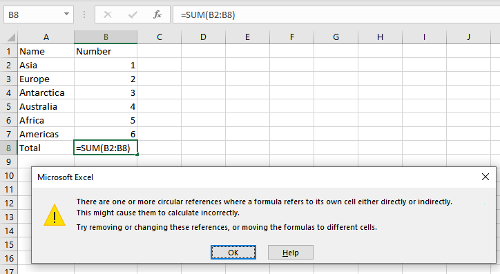
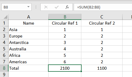
- The formula in cell B8 refers to itself. When the user applies a function such as a sum or manually uses the reference of B8, a direct circular reference warning is displayed.
- Once the warning shows up, the user can click on OK, but it will only result in zero.
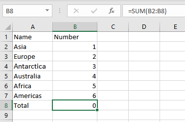
This is an example of a direct circular reference in Excel.
Indirect Circular Reference
As the name suggests, an indirect circular reference takes place when a value in a formula refers to its cell, not directly but at some level. See the simple example below for a better understanding.
For creating an indirect circular reference example, we will have to write a chain of formulas using values starting from the first cell.
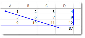
- For example, the data is populated in a way where the diagonals are squares of the previous diagonals as you can see.
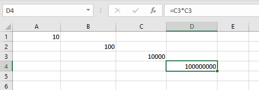
- Now the data is starting from A1 which has the value 10 and every other diagonal till D4 is dependent on A1. If the user uses a reference of any diagonal in A1, it will create a circular reference warning. Let’s try it out.
- As seen in the screenshot below, Excel goes as far as creating a linked line showing the Precedents and Dependents.
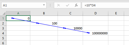
- It results in a value of 0 since it is a circular reference issue.
Now, let’s try to see and understand how to find circular reference issues in excel.
How to Find Circular References in Excel
While you will get the circular reference warning when it occurs, however, you will still need to figure out in which cell the error has occurred. After knowing the exact cell location of the error it will be easier to handle and fix it.
These methods are particularly helpful when you are working with large datasets.
1) Error Checking drop-down in the Ribbon
Here’s how you can find circular references in Excel using the Ribbon.
- Open the worksheet where the circular reference has occurred.
- Go to the Formulas tab and click on the Error Checking drop-down menu.
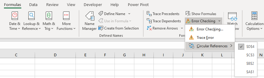
- Select Circular References from the drop-down menu.
- Here Excel will show you all the circular references that are in the worksheet.
- Click on whichever circular reference you want and it will take you to that particular cell to solve the issue.
As you can see in the screenshot above, there are 4 circular references in the worksheet that we are using.
2) Using Status bar
Finding circular references using the status bar is very easy. If a circular reference exists in the worksheet, the user will be able to see it in the status bar below the worksheet names.
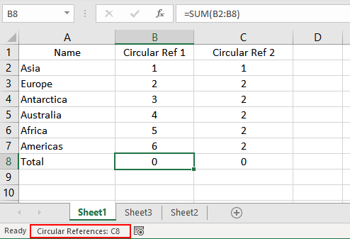
Note: It only shows the latest circular reference and the user can backtrack from there. As seen in the example below, there are two circular references notably in B8 and C8 but the status bar only shows C8.
Iterative Calculations
Iterative calculations are an interesting feature in Excel. What iterative calculations mean is that if the user keeps them disabled as they usually are, Excel returns a Circular Reference prompt and returns a 0 in the cell instead of the actual result. This is because it is an endless loop.
Now, the thing is that if you want to tell Excel to sit out and let you do your job without bothering you about those pesky circular reference warnings, you can enable Iterative Calculations and it will allow you to perform your calculations. Not only that, but it will also allow you to set a fixed number of maximum iterations.
If you wish to enable iterative calculations, you can set the number of iterations allowed. Hence, you can stop the circular reference infinite loops and can have a tiny bit of control over such calculations.
How to Enable/Disable Iterative Calculations in Excel
Now that we have established how iterative calculations work, let’s show you how you can enable or disable iterative calculations in Excel. Follow the below steps to enable or disable iterative calculations in excel.
- Go to the File tab.
- Click on Options.
- The Excel Options dialog box will open. Click on Formulas from the left column.
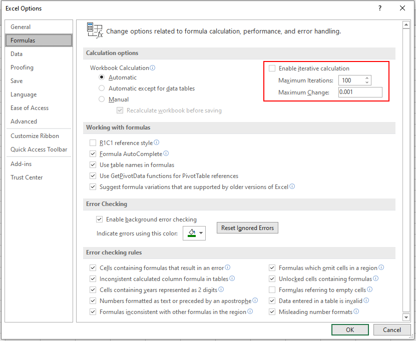
- Here, the option to Enable Iterative Calculation is available. Users can simply tick the box to enable. The user is also able to set maximum iterations and maximum change.
- After enabling iterative calculation, you will see that the calculation will not result in 0 but will produce results in case of circular reference as you can see.
Maximum Iterations & Maximum Change Parameters
The two parameters of the Iterative Calculations are:
Maximum iterations: This is the loop that Excel will run when it is calculating the final result. You can set this as you want. Remember that more iterations mean more processing for Excel which will in turn use more resources and processing power from the computer. It would also take more time.
Maximum change: The maximum change is the value that needs to be achieved in order for the iteration to move further. It is about the accuracy of the result. Make this value small as it will produce accurate results. The default Maximum Change is 0.001.
Deliberately Using Circular References
The deliberate use of Circular references is not a very good idea, though sometimes it can help you to get away with poorly developed logic or formulas. But doing this is not recommended at all. However, for educational purposes let’s try and understand how to get things working with deliberate circular references.
The first step is to enable Iterative Calculation in Excel. Once you have turned on Iterative Calculation and set your maximum iterations, you can start using circular references to your benefit.
Let us demonstrate that by using an example.
Let’s say that the user requires to manipulate the data in a way that two cells depend on each other for values causing a circular reference issue. Since the iterative calculation is enabled, there won’t be a prompt.
In the example below, the cells B4 and B5 depend on each other, creating a circular reference. Since the iterative calculation is enabled, there will not be an error or a 0 in the results. Instead, Excel will try calculating the results.
In the example, the Agent fee is 20% of the total earnings of the player. Since the total earning and agent fee are dependent on each other, it can still be calculated if iterative calculation is enabled.
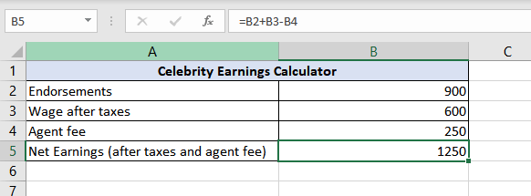
To use it as we see fit, we must first apply our desired formula in the net earnings cell.
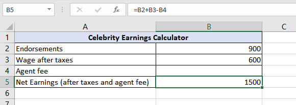
Now the Agent fee must be calculated which we are going to set at 20% of total earnings but the total earnings will then have to subtract the Agent fee from itself, hence the circular reference.
As you can see, it works perfectly.
Why Should We Avoid Using Circular References Deliberately?
Using Circular References in Excel is not recommended at all. Deliberate use of circular references is a slippery method to make things work that eats up a lot of resources and processing power when being used with iterative calculations. It can often produce undesired or inaccurate results that can cause frustration when you have to fix a few of them.
How to fix Circular References in Excel
Fixing circular references in Excel is not possible with a single click. To handle circular references, you have to eliminate them one by one. You can trace it back to the source and remove the starting formula to fix it, or you can remove it one by one.
There are two tracing methods that will allow you to remove circular references by tracing relationships between formulas and cells.
To access the tracing methods, you have to follow the following steps:
- Go to the Formulas tab in Excel
- The Trace Precedents and Trace Dependents options are available there.

These tracing features can help the user in fixing circular references by providing a path connecting the references through a line that is drawn between cells that are responding to the circular references.
The two tracing options work as follows:
Trace Precedents
The trace precedents feature tracks back cells that the current cell depends on. These are the cells on which the current formula is dependent for the data that it needs. This option will draw lines that will tell which cells are affecting the active cell.
In the example below, the cells affecting B5 are B2, B3, and B4. Hence, when we click on Trace Precedents, it draws a line indicating B2, B3, and B5 cells leading to B5.
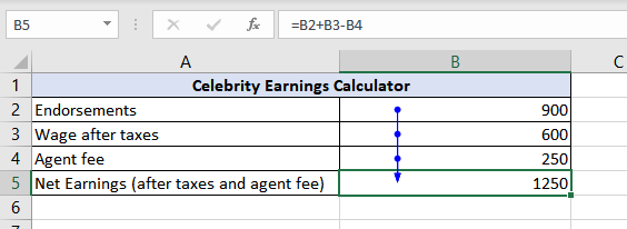
Shortcut for Trace Precedents: ALT + T U T
Trace Dependents
The trace dependents feature tracks the cells that are dependent on the active cell, the cells that depend on the current cell for the data they need to produce results. This feature will draw lines to the cells that are dependent on the active cell.
In the example below, the cell being affected by B5 is B4. It is dependent on B5 for its value. Hence, when we use trace dependents, it draws a line from B5 to B4, indicating that B4 is dependent on B5.
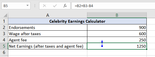
Shortcut for Trace Dependents: ALT + T U D
So, this was all about circular references in Excel. Hopefully, by now, you have a good idea of how circular references work, how you can find/fix them, and how you can use them if you desire.
The circular reference error in Excel, is a very common error that can occur when using almost any formula. When you see the circular reference error displayed in your Excel spreadsheet, this means that your formula is referring to a range that contains the formula itself, or in other words when the formula input, is dependent on the output.
To fix the circular reference in Excel, make either of the following changes to your spreadsheet:
- Move your formula to another cell that is not contained within the range(s) that the formula refers to
- Or, adjust the reference in your formula so that it does not refer to a range that contains the formula itself
There are several different ways that a circular reference may display an error / warning in Excel:
- Some versions of Excel will display a pop up warning, that has a message like this: «There are one or more circular references where a formula refers to its own cell either directly or indirectly. This might cause them to calculate incorrectly. Try removing or changing these references, or moving the formulas to different cells»
- In some versions, the warning may say this «Careful, we found one or more circular references in your workbook that might cause your formula to calculate incorrectly. FYI: A circular reference can be a formula that refers to its own cell value, or refers to a cell dependent on its own cell value.
- In some versions of Excel (such as Excel online), the cell will sometimes not display a warning, and will simply calculate incorrectly, where the number «0» displays as the formula result
- In some cases, such as when using the FILTER function, a circular reference can cause an «Empty Array» warning / error
Since I used Excel Online to create these examples, most of my examples show the third error in the list above, where the cell shows the number 0. The error may appear differently on your version of Excel, but the cause of the error as well as the solution are the same across the board.
This article shows how to fix a circular reference error in Excel, but click here if you want to learn how to fix the circular dependency error in Google Sheets.
Circular reference errors can also occur when two formulas refer to the range that the other formula resides in, even if the formula does not refer to itself (i.e. its own location). In the same way that a single formula’s input cannot be dependent on data that is determined by its own output, two formulas cannot simultaneously be dependent on each other’s output. This can cause a confusing situation where one wrong formula causes two formula errors.
In this article I will go over several different examples of how you might experience this reference error in Excel, and I will also show you how to fix the error in each situation.
When a circular reference error occurs in your spreadsheet, the cell that contains the formula error will either display the number 0, or Excel may display a warning / error, or both.
Below are two examples of the circular reference warning that you might see:

When your formula is inside of the range that it is referring to, this means that the formula input is «dependent» on the output, which is not possible to calculate, and causes an error.
Question 1: Divide 10 by the answer to question 1.
This is impossible to solve because the output/answer cannot be known before the problem is actually solved.
Or in the case of two formulas that refer to each other’s output/location, here is another analogy. This is like being given the two following math problems:
Question 1: What is the answer to question 2?
Question 2: What is the answer to question 1?
Again, this cannot be solved. The answer to each question is dependent on the other, which makes your mind run in circles… hence the phrase «circular reference».
Don’t let this make you feel confused, because that’s the point is that this logic causes an error. All you need to know is why it happens, and how to fix it.
So let’s go over some actual examples of resolving this circular reference error in your Excel spreadsheet.
Let’s take a look at the most simple example of the circular reference error.
Below, the image shows a formula that simply refers to a single cell. However, the problem is that the cell that formula is referring to, is the cell that the formula is entered into (the formula in cell A1, is referring to cell A1).
As you can see, this has caused a circular reference error.
The following formula causes an error, when entered into cell A1:
=A1
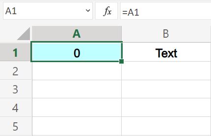
To fix the error, we can either move the formula to another cell, or change the reference in the formula so that it refers to another cell.
In this case we will change the cell reference to cell B1.
As you can see in the image below, this adjustment has fixed the circular reference error.
The following formula has been adjusted and resolves the error:
=B1
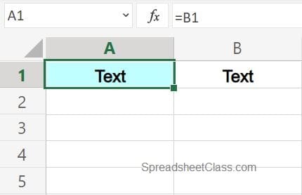
Now, cell A1 displays the text that is in cell B1.
Fixing circular reference when summing
A common situation where you might experience the circular reference error, is when you are summing in Excel. This will happen most often when your SUM formula is in the same column that it refers to, and when the formula reference captures the entire column.
The image below shows a simple SUM formula, that attempts to sum the numbers in cells A1 through A5.
But as you can see, the SUM formula refers to the range A1:A10. Since the SUM formula is entered into a cell within column A (A6), and the range A1:A10 contains cell A6 (where the formula is), this causes a circular reference error.
The following formula causes an error when entered anywhere in column A:
=SUM(A1:A10)
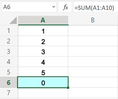
To fix this error, we will adjust the reference in the formula so that it only sums the values in the cells above it.
So rather than trying to sum the entire column, we will designate an ending row in the reference (a row that is above the sum formula).
To do this, simply change the sum range to A1:A5.
This fixes the circular reference error, as shown in the image below.
The following formula has been adjusted and resolves the error:
=SUM(A1:A5)
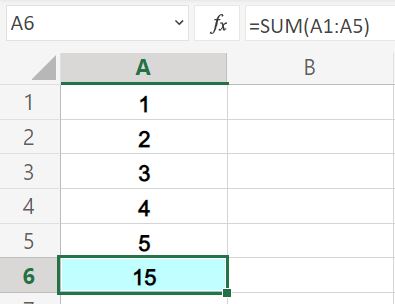
Now the SUM formula in the image above, successfully sums cells A1 through A5. (1+2+3+4+5=15)
Fixing circular reference when filtering
In the last example we had to adjust the rows in the formula reference to fix the circular reference error, but let’s take a look at an example where we will adjust the columns in the reference to resolve the error.
In this example, let’s say that we have a list of school supplies and their prices entered into a spreadsheet, and we want to filter the data with a formula so that a list of items costing more than $1 is displayed.
As you can see in the image below, the FILTER formula has a circular reference error. This is being caused by the reference to the source range, which is one column too wide (considering where the filter formula has been placed).
If the formula refers to the range A2:D, which contains column D, the formula cannot be placed in column D.
The following formula causes an error when entered into cell D2:
=FILTER(A2:D10,C2:C10>1)
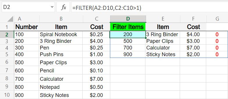
To fix the error that is shown in the image above, change the range that refers to the source data from A2:D10, to A2:C10.
After making this adjustment, the error is fixed, and the FILTER formula works properly.
The following formula has been adjusted and resolves the error:
=FILTER(A2:C10,C2:C10>1)
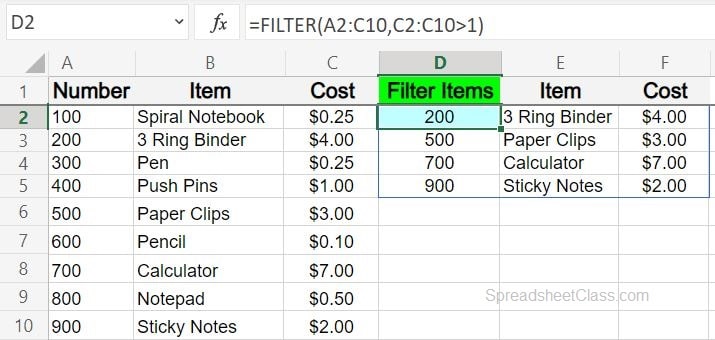
Now the school supplies are being filtered to display a list of items that cost more than $1.
This content was originally created and written by SpreadsheetClass.com
Fixing circular reference with if/then statement
Now let’s take a look at a more complex example, that could happen to anyone who uses formulas in their spreadsheets. In this example, there are two different formulas that are interacting, and because one of them was set up incorrectly, both are displaying an error, due to the fact that each are referring to (dependent on) each other.
(For more explanation on why this happens, see the top of this article)
When an error happens like the one that is shown in the image below, it can sometimes be hard to determine which formula has the mistake, because of the double error that it causes. As in any troubleshooting scenario… the best thing to do is to start from the beginning, and trace your way through the data/system until you find the mistake.
So here is the scenario in this example: Column A indicates the completion of a task with 1’s and 0’s. The formulas in column B were intended to refer to the data in column A, and to display the text «Yes» or «No», depending on if each cell in column A had a number 1 or a number 0. Then, column C refers to the cells in column B, and displays the words «Complete» or » Not Complete», depending on whether each cell in column B says yes or no.
In short, if cell A3 contains the number 1, then cell B3 should say «Yes», and cell C3 should say «Complete».
But the problem is that the formula in cell B3… instead of referring to the 1’s and 0’s in column A, the sheet’s creator made a mistake, and referred to column C (which in turn is referring back to it). This creates a circular reference error, in BOTH formulas, even though technically only one of the formulas was set up incorrectly.
This type of mix up is common when using lots of formulas in your sheets, and especially when you have been creating all day and are tired.
To fix this formula, which will fix both of the circular reference errors, follow the instructions listed below the image.
The following formula causes an error when entered into cell B3, due to another formula in cell C3 that refers to cell B3:
=IF(C3=»Complete»,»Yes»,»No»)
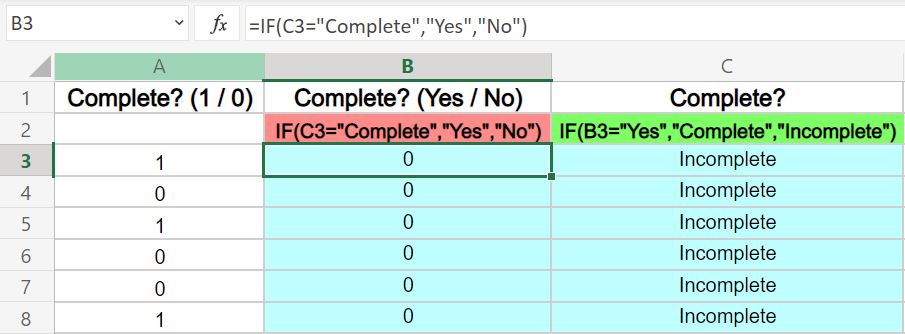
In this case, to fix the error, it is more than just a matter of changing the reference in the formula, because the whole formula was written incorrectly by mistake. So remember that the formulas in column B, should display the word «Yes» in each row/cell if there is a number 1 in the adjacent cells in column A (and the word «No» if there is a 0 in the adjacent cell).
The corrected logic for the formula in cell B3, is as follows: If cell A3 equals 1, then display the word «Yes», and if not, then display the word «No».
The following formula has been adjusted and resolves the error:
=IF(A3=1,»Yes»,»No»)
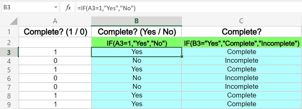
Now both of the formulas are working properly, and both of the circular reference errors have been fixed at the same time, by correcting one formula.
Now, column B refers to column A, and then column B refers to column C, as it should be. The formulas are no longer simultaneously dependent on each other’s output.
Fix the circular reference error when referring to another tab
One more very common way of running into the circular reference error, is when you are referring to another tab in your formula, and you forget to include the tab name in your reference.
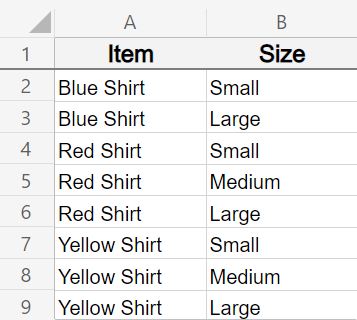
The data below shows a list of clothing items and their sizes listed in a spreadsheet. We want to filter the data by using a formula in another tab, to only show items that have the size «Medium».
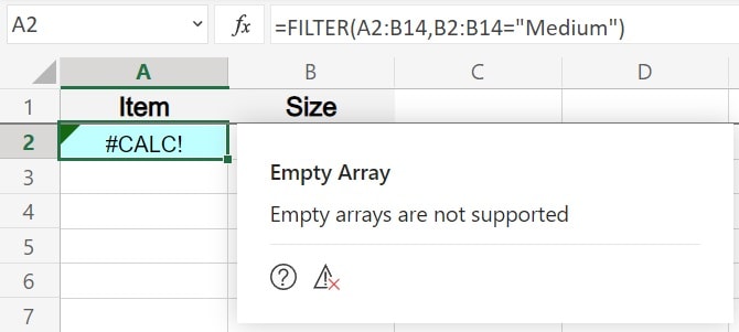
The picture below shows a FILTER formula that is entered in cell A2, on a different tab than the one that holds the source data shown above.
The problem is that the tab name was left out when the formula was entered.
Since the source range is A2:B14 and the formula is in cell A2, this means that the formula is referring to itself. Or in other words, the cell that the formula is entered in, is within the range that the formula refers to. This causes a circular reference error.
The following formula causes an error when entered into cell A2:
=filter(A2:B14,B2:B14=»Medium»)
To fix this error, simply add the tab name to the references in the filter formula.
The reference to the source range will be ‘Another Tab’!A2:B14 (Apostrophes must be added before and after the tab name reference, when there is a space in the tab name).
The following formula has been adjusted and resolves the error:
=filter(‘Another Tab’!A2:B14,’Another Tab’!B2:B14=»Medium»)
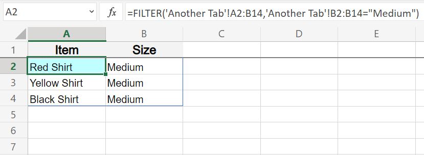
After adding the tab name to the references in the FILTER formula, the circular reference error goes away, and the formula filters properly, displaying a list of clothing items that are «Medium».
Now you know how to easily fix this error whenever it pops up in your spreadsheet!
By manually moving the formula you can solve this issue
by Teodor Nechita
Eager to help those in need, Teodor writes articles daily on subjects regarding Windows, Xbox, and all things tech-related. When not working, you may usually find him either… read more
Updated on January 20, 2023
Reviewed by
Vlad Turiceanu

Passionate about technology, Windows, and everything that has a power button, he spent most of his time developing new skills and learning more about the tech world. Coming… read more
- Microsoft Excel is one of the most important spreadsheet tools in the world.
- The article below will show you how to solve all circular reference errors that you may encounter in Excel.
This article will be covering an issue that many users have reported on forums, regarding a particular Microsoft Excel issue:
I keep getting this error upon startup of a spreadsheet i made. I must have made an invalid formula somewhere but can’t seem to find it at all. Is there a way i can easily find the error and prevent this annoying message from popping up every time? Also, I notice this spreadsheet takes WAYYY too long to start up. Not sure if there’s a fix for that too.
For those of you that don’t know, a circular reference means that your formula is trying to calculate itself since you are referring to cells already included in the formula.
The full message reads as follows:
There are one or more circular references where a formula refers to its own cell either directly or indirectly. This might cause them to calculate incorrectly. Try removing or changing these references, or moving the formulas to different cells.
Further research revealed that this is a common error message, so we decided to make a list of the best ways you can overcome the circular reference error in Microsoft Excel.
How do I fix the circular reference error in Microsoft Excel?
1. Enable the iterative calculation feature
If you want a workaround for the circular reference error in Excel, you should enable the iterative calculation feature. By doing so, you will be able to use circular references without encountering any issues. Here is how to do so:
1. Open Microsoft Excel.
2. Select File and go to Options.
3. Select Formulas.
4. Check the box next to Enable iterative calculation.
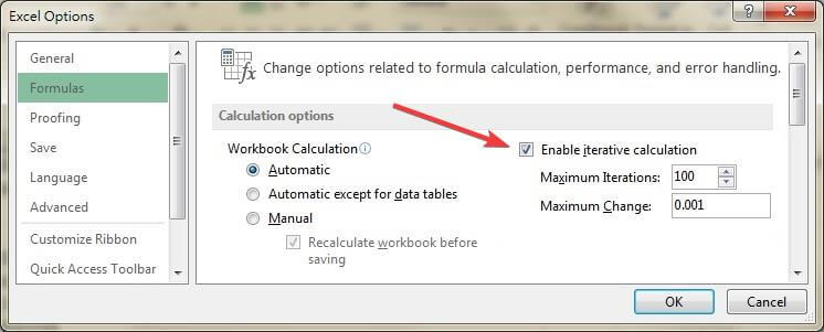
5. Click Ok to apply and save the changes.
2. Find the cell causing the circular reference error
- Launch Microsoft Excel
- Trigger the error message
- Go to the Formulas tab
- Select Errors Checking

- Select the Circular Reference entry
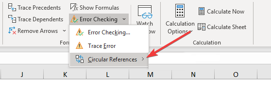
- This will automatically fix any reference errors
3. Manually move the formula to another cell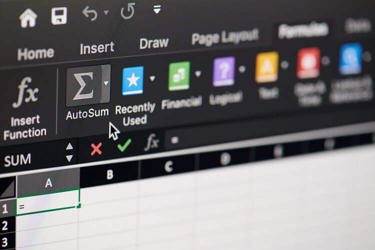
If you have a simple calculation, for example, A1 + A2 + A3= A4, but you wanted to put the SUM formula on A1, A2, or A3 instead of A4, this will trigger the reference error.
That being the case, simply choose a different cell for your formula, without overlapping with the cells that already have numerical values inside of them.
By following the steps below, you should be able to fix any circular reference error and resume using Microsoft Excel accordingly.
Which one of the methods worked best for you? Let us know by leaving us a message in the comments section below.
Still having issues? Fix them with this tool:
SPONSORED
If the advices above haven’t solved your issue, your PC may experience deeper Windows problems. We recommend downloading this PC Repair tool (rated Great on TrustPilot.com) to easily address them. After installation, simply click the Start Scan button and then press on Repair All.

Newsletter
While working with Excel formulas, you may sometime see the following warning prompt.
This prompt tells you that there is a circular reference in your worksheet and this can lead or an incorrect calculation by the formulas. It also asks you to address this circular reference issue and sort it.
In this tutorial, I will cover all that you need to know about circular reference, and well as how to find and remove circular references in Excel.
So let’s get started!
What is Circular Reference in Excel?
In simple words, a circular reference happens when you end up having a formula in a cell – which in itself uses the cell (in which it’s been entered) for the calculation.
Let me try and explain this by a simple example.
Suppose you have the dataset in cell A1:A5 and you use the below formula in cell A6:
=SUM(A1:A6)
This will give you a circular reference warning.
This is because you want to sum the values in cell A1:A6, and the result should be in cell A6.
This creates a loop as Excel just keeps on adding the new value in cell A6, which keeps on changing (hence, a circular reference loop).
How to Find Circular References in Excel?
While the circular reference warning prompt is kind enough to tell you that it exists in your worksheet, it doesn’t tell you where it’s happening and what cell references are causing it.
So if you’re trying to find and handle circular references in the worksheet, you need to know a way to somehow find these.
Below are the steps to find a circular reference in Excel:
- Activate the worksheet that has the circular reference
- Click the Formulas tab
- In the Formula Editing group, click on the Error Checking drop-down icon (little downward pointing arrow at the right)
- Hover the cursor over the Circular References option. It will show you the cell that has a circular reference in the worksheet
- Click on the cell address (that is displayed) and it will take you to that cell in the worksheet.
Once you have addressed the issue, you can again follow the same steps above and it will show more cell references that have the circular reference. If there is none, you will not see any cell reference,
Another quick and easy way to find the circular reference is by looking at the Status bar. On the left part of it, it will show you the text Circular Reference along with the cell address.
There are a few things you need to know when working with circular references:
- In case the iterative calculation is enabled (covered later in this tutorial), the status bar will not show the circular reference cell address
- In case the circular reference is not in the active sheet (but in other sheets in the same workbook), it will only show Circular reference and not the cell address
- In case you get a circular reference warning prompt once and you dismiss it, it will not show the prompt again the next time.
- If you open a workbook that has the circular reference, it will show you the prompt as soon as the workbook opens.
How to Remove a Circular Reference in Excel?
Once you have identified that there are circular references in your sheet, it’s time to remove these (unless you want them to be there for a reason).
Unfortunately, it’s not as simple as hitting the delete key. Since these are dependent on formulas and every formula is different, you need to analyze this on a case-by-case basis.
In case it’s just a matter of having the cell reference causing the issue by mistake, you can simply correct by adjusting the reference.
But sometimes, it’s not that simple.
Circular reference can also be caused based on multiple cells that feed into each other at many levels.
Let me show you an example.
Below there is a circular reference in cell C6, but it’s not just a simple case of self-reference. It’s multi-level where the cells it uses in the calculations also reference each other.
- The formulas in cell A6 is =SUM(A1:A5)+C6
- The formula is cell C1 is =A6*0.1
- The formula in cell C6 is =A6+C1
In the above example, the result in cell C6 is dependent on the values in cell A6 and C1, which in turn are dependent on cell C6 (thus causing the circular reference error)
And again, I have chosen a really simple example just for demo purposes. In reality, these could be quite difficult to figure out and maybe far off in the same worksheet or even scattered across multiple worksheets.
In such a case, there is one way to identify the cells that are causing circular reference and then treat these.
It’s by using the Trace Precedents option.
Below are the steps to use trace precedents to find cells that are feeding to the cell that has the circular reference:
- Select the cell that has the circular reference
- Click the Formulas tab
- Click on Trace Precedents
The above steps would show you blue arrows which will tell you what cells are feeding into the formula in the selected cell. This way, you can inspect the formulas and the cells and get rid of the circular reference.
In case you’re working with complex financial models, it may be possible that these precedents also go multiple levels deep.
This works well if you have all the formulas referring to cells in the same worksheet. If it’s in multiple worksheets, this method is not effective.
How to Enable/Disable Iterative Calculations in Excel
When you have a circular reference in a cell, first you get the warning prompt as shown below, and if you close this dialog box, it will give you 0 as the result in the cell.
This is because when there is a circular reference, it’s an endless loop and Excel doesn’t want to caught up in it. So it returns a 0.
But in some cases, you may actually want the circular reference to be active and do a couple of iterations. In such a case, instead of an infinite loop, and you can decide how many times the loop should be run.
This is called iterative calculation in Excel.
Below are the steps to enable and configure iterative calculations in Excel:
- Click the File tab
- Click on Options. This will open the Excel Options dialog box
- Select Formula in the left pane
- In the Calculation options section, check the box ‘Enable iterative calculation’. Here you can specify the maximum iterations and maximum change value
That’s it! The above steps would enable iterative calculation in Excel.
Let me also quickly explain the two options in the iterative calculation:
- Maximum iterations: This is the maximum number of times you want Excel to calculate before giving you the final result. So if you specify this as 100, Excel will run the loop 100 times before giving you the final result.
- Maximum Change: This is the maximum change, which if not achieved between iterations, the calculation would be stopped. By default, the value is .001. The lower this value, the more accurate would be the result.
Remember that the more number of times the iterations run, the more time and resources it takes for Excel to do it. In case you keep the maximum iterations high, it may lead to your Excel slowing down or crashing.
Note: When iterative calculations are enabled, Excel will not show you the circular reference warning prompt and will also now show it in the status bar.
Deliberately Using Circular References
In most cases, the presence of circular reference in your worksheet would be an error. And this is why Excel shows you a prompt which says – “Try removing or changing these references or moving the formulas to different cells.”
But there might be some specific cases where you need a circular reference so that you can get the desired result.
One such specific case I have already written about it getting the time stamp in a cell in a cell in Excel.
For example, suppose you want to create a formula so that every an entry is made in a cell in Column A, the timestamp appear in Column B (as shown below):
While you can insert easily insert a timestamp using the below formula:
=IF(A2<>"",IF(B2<>"",B2,NOW()),"")
The issue with the above formula is that it would update all the timestamps as soon as any change is made in the worksheet or if the worksheet is reopened (as the NOW formula is volatile)
To get around this issue, you can use a circular reference method. Use the same formula, but enable iterative calculation.
There are some other cases as well where having the ability to use circular reference is desired (you can find one example here).
Note: While there may be some cases where you can use circular reference, I find it best to avoid using it. Circular references can also take a toll on the performance of your workbook and can make it slow. In rare cases where you need it, I always prefer using VBA codes to get the work done.
I hope you found this tutorial useful!
Other Excel tutorials you may find useful:
- #REF! Error in Excel; How to Fix the Reference Error!
- Excel VBA Error Handling
- Use IFERROR with VLOOKUP to Get Rid of #N/A Errors
- How to Reference Another Sheet or Workbook in Excel (with Examples)
- Absolute, Relative, and Mixed Cell References in Excel
This article will address a problem that many users Reported on the forums regarding a specific Microsoft Excel issue:
I keep getting this error when running a spreadsheet I made. I must have done the wrong formula somewhere, but I can’t seem to find it at all. Is there a way I can easily find the error and prevent this annoying message from appearing every time? Also, I’ve noticed that this spreadsheet takes a VERY long time to run. Not sure if there is a fix for this too.
For those of you who don’t know, a circular reference means that your formula is trying to evaluate itself because you are referencing cells already included in the formula.
The full message is:
There is one or more circular references in which the formula directly or indirectly refers to its own cell. This may cause them to be miscalculated. Try removing or changing these links, or move the formulas to other cells.
Further research has shown that this is a common error message, so we decided to compile a list of the best ways to overcome the circular reference error in Microsoft Excel.
How to fix circular reference error in Microsoft Excel?
Enable iterative calculation feature
If you need a workaround for the circular reference error in Excel, you should enable the iterative calculation feature. This way you will be able to use circular references without any problems. Here’s how to do it:
1. Open Microsoft Excel.
2. Select «File» and go to «Options».
3. Select formula.
4. Check the box next to Enable iterative calculation.
5. Click «OK»to apply and save your changes.
Find the cell causing the circular reference error
- Run Microsoft Excel
- Raise an error message
- Click the tab formula
- Select an entry Circular link

- This will automatically fix any reference errors
Manually move formula to another cell
If you have a simple calculation like A1 + A2 + A3= A4, but you want to put the SUM formula on A1, A2, or A3 instead of A4, this will throw a link error.
In this case, just select a different cell for your formula without overlapping cells that already have numeric values.
By following the steps below, you should be able to fix any circular reference error and resume using Microsoft Excel accordingly. Which method worked best for you? Let us know by leaving us a message in the comments section below.