Табличные значения функции ошибок

Таблица значений функции Лапласа

В таблице даны значения функции

для положительных значений

и для

;
для

пользуются той же таблицей, так как функция

нечетна, то есть

.
В таблице приведены значения интеграла лишь до

,
так как для

можно принять

.
Эту функцию называют функцией Лапласа.

Таблица значений функции Лапласа в теории вероятностей и математической статистике используется довольно часто. На сайте можно посмотреть примеры ее использования в следующих задачах:

Отклонение относительной частоты от постоянной вероятности в независимых испытаниях
Интегральная теорема Муавра – Лапласа
Доверительные интервалы для среднего и дисперсии
Проверка гипотезы о равенстве средних

Цветом в таблице подсвечены аргументы функции Лапласа, рядом, в соседнем столбце — значения функции Лапласа.

x	Ф(x)	x	Ф(x)	x	Ф(x)	x	Ф(x)
0,00	0,0000	0,32	0,1255	0,64	0,2389	0,96	0,3315
0,01	0,0040	0,33	0,1293	0,65	0,2422	0,97	0,3340
0,02	0,0080	0,34	0,1331	0,66	0,2454	0,98	0,3365
0,03	0,0120	0,35	0,1368	0,67	0,2486	0,99	0,3389
0,04	0,0160	0,36	0,1406	0,68	0,2517	1,00	0,3413
0,05	0,0199	0,37	0,1443	0,69	0,2549	1,01	0,3438
0,06	0,0239	0,38	0,1480	0,70	0,2580	1,02	0,3461
0,07	0,0279	0,39	0,1517	0,71	0,2611	1,03	0,3485
0,08	0,0319	0,40	0,1554	0,72	0,2642	1,04	0,3508
0,09	0,0359	0,41	0,1591	0,73	0,2673	1,05	0,3531
0,10	0,0398	0,42	0,1628	0,74	0,2703	1,06	0,3554
0,11	0,0438	0,43	0,1664	0,75	0,2734	1,07	0,3577
0,12	0,0478	0,44	0,1700	0,76	0,2764	1,08	0,3599
0,13	0,0517	0,45	0,1736	0,77	0,2794	1,09	0,3621
0,14	0,0557	0,46	0,1772	0,78	0,2823	1,10	0,3643
0,15	0,0596	0,47	0,1808	0,79	0,2852	1,11	0,3665
0,16	0,0636	0,48	0,1844	0,80	0,2881	1,12	0,3686
0,17	0,0675	0,49	0,1879	0,81	0,2910	1,13	0,3708
0,18	0,0714	0,50	0,1915	0,82	0,2939	1,14	0,3729
0,19	0,0753	0,51	0,1950	0,83	0,2967	1,15	0,3749
0,20	0,0793	0,52	0,1985	0,84	0,2995	1,16	0,3770
0,21	0,0832	0,53	0,2019	0,85	0,3023	1,17	0,3790
0,22	0,0871	0,54	0,2054	0,86	0,3051	1,18	0,3810
0,23	0,0910	0,55	0,2088	0,87	0,3078	1,19	0,3830
0,24	0,0948	0,56	0,2123	0,88	0,3106	1,20	0,3849
0,25	0,0987	0,57	0,2157	0,89	0,3133	1,21	0,3869
0,26	0,1026	0,58	0,2190	0,90	0,3159	1,22	0,3883
0,27	0,1064	0,59	0,2224	0,91	0,3186	1,23	0,3907
0,28	0,1103	0,60	0,2257	0,92	0,3212	1,24	0,3925
0,29	0,1141	0,61	0,2291	0,93	0,3238	1,25	0,3944
0,30	0,1179	0,62	0,2324	0,94	0,3264
0,31	0,1217	0,63	0,2357	0,95	0,3289

Если не находите примера, аналогичного вашему, если сами не успеваете выполнить работу, если впереди экзамен по предмету и нужна помощь — свяжитесь со мной:

ВКонтакте
WhatsApp
Telegram

Я буду работать с вами, над вашей проблемой, пока она не решится.

Продолжение таблицы

x	Ф(x)	x	Ф(x)	x	Ф(x)	x	Ф(x)
1,26	0,3962	1,59	0,4441	1,92	0,4726	2,50	0,4938
1,27	0,3980	1,60	0,4452	1,93	0,4732	2,52	0,4941
1,28	0,3997	1,61	0,4463	1,94	0,4738	2,54	0,4945
1,29	0,4015	1,62	0,4474	1,95	0,4744	2,56	0,4948
1,30	0,4032	1,63	0,4484	1,96	0,4750	2,58	0,4951
1,31	0,4049	1,64	0,4495	1,97	0,4756	2,60	0,4953
1,32	0,4066	1,65	0,4505	1,98	0,4761	2,62	0,4956
1,33	0,4082	1,66	0,4515	1,99	0,4767	2,64	0,4959
1,34	0,4099	1,67	0,4525	2,00	0,4772	2,66	0,4961
1,35	0,4115	1,68	0,4535	2,02	0,4783	2,68	0,4963
1,36	0,4131	1,69	0,4545	2,04	0,4793	2,70	0,4965
1,37	0,4147	1,70	0,4554	2,06	0,4803	2,72	0,4967
1,38	0,4162	1,71	0,4564	2,08	0,4812	-2,74	0,4969
1,39	0,4177	1,72	0,4573	2,10	0,4821	2,76	0,4971
1,40	0,4192	1,73	0,4582	2,12	0,4830	2,78	0,4973
1,41	0,4207	1,74	0,4591	2,14	0,4838	2,80	0,4974
1,42	0,4222	1,75	0,4599	2,16	0,4846	2,82	0,4976
1,43	0,4236	1,76	0,4608	2,18	0,4854	2,84	0,4977
1,44	0,4251	1,77	0,4616	2,20	0,4861	2,86	0,4979
1,45	0,4265	1,78	0,4625	2,22	0,4868	2,88	0,4980
1,46	0,4279	1,79	0,4633	2,24	0,4875	2,90	0,4981
1,47	0,4292	1,80	0,4641	2,26	0,4881	2,92	0,4982
1,48	0,4306	1,81	0,4649	2,28	0,4887	2,94	0,4984
1,49	0,4319	1,82	0,4656	2,30	0,4893	2,96	0,4985
1,50	0,4332	1,83	0,4664	2,32	0,4898	2,98	0,4986
1,51	0,4345	1,84	0,4671	2,34	0,4904	3,00	0,49865
1,52	0,4357	1,85	0,4678	2,36	0,4909	3,20	0,49931
1,53	0,4370	1,86	0,4686	2,38	0,4913	3,40	0,49966
1,54	0,4382	1,87	0,4693	2,40	0,4918	3,60	0,499841
1,55	0,4394	1,88	0,4699	2,42	0,4922	3,80	0,499928
1,56	0,4406	1,89	0,4706	2,44	0,4927	4,00	0,499968
1,57	0,4418	1,90	0,4713	2,46	0,4931	4,50	0,499997
1,58	0,4429	1,91	0,4719	2,48	0,4934	5,00	0,499997

Пример решения задачи

Задача

Вероятность того, что
желание, загаданное на Новый год, сбудется, равна 0,7. Найти вероятность того,
что из 100 загаданных желаний сбудется от 60 до 85 желаний.

Решение

Вероятность того, что
событие

появится в

независимых
испытаниях от

до

раз:

В нашем случае

По таблице функции
Лапласа:

Искомая вероятность:

Источник

Error function
Plot of the error function
General information
General definition	${displaystyle operatorname {erf} z={frac {2}{sqrt {pi }}}int _{0}^{z}e^{-t^{2}},mathrm {d} t}$
Fields of application	Probability, thermodynamics
Domain, Codomain and Image
Domain	$mathbb {C}$
Image	${displaystyle left(-1,1right)}$
Basic features
Parity	Odd
Specific features
Root	0
Derivative	${displaystyle {frac {mathrm {d} }{mathrm {d} z}}operatorname {erf} z={frac {2}{sqrt {pi }}}e^{-z^{2}}}$
Antiderivative	${displaystyle int operatorname {erf} z,dz=zoperatorname {erf} z+{frac {e^{-z^{2}}}{sqrt {pi }}}+C}$
Series definition
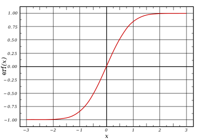
Taylor series	${displaystyle operatorname {erf} z={frac {2}{sqrt {pi }}}sum _{n=0}^{infty }{frac {z}{2n+1}}prod _{k=1}^{n}{frac {-z^{2}}{k}}}$

In mathematics, the error function (also called the Gauss error function), often denoted by erf, is a complex function of a complex variable defined as:^[1]

${displaystyle operatorname {erf} z={frac {2}{sqrt {pi }}}int _{0}^{z}e^{-t^{2}},mathrm {d} t.}$

This integral is a special (non-elementary) sigmoid function that occurs often in probability, statistics, and partial differential equations. In many of these applications, the function argument is a real number. If the function argument is real, then the function value is also real.

In statistics, for non-negative values of x, the error function has the following interpretation: for a random variable Y that is normally distributed with mean 0 and standard deviation 1/√2, erf x is the probability that Y falls in the range [−x, x].

Two closely related functions are the complementary error function (erfc) defined as

${displaystyle operatorname {erfc} z=1-operatorname {erf} z,}$

and the imaginary error function (erfi) defined as

${displaystyle operatorname {erfi} z=-ioperatorname {erf} iz,}$

where i is the imaginary unit

Name[edit]

The name «error function» and its abbreviation erf were proposed by J. W. L. Glaisher in 1871 on account of its connection with «the theory of Probability, and notably the theory of Errors.»^[2] The error function complement was also discussed by Glaisher in a separate publication in the same year.^[3]
For the «law of facility» of errors whose density is given by

${displaystyle f(x)=left({frac {c}{pi }}right)^{frac {1}{2}}e^{-cx^{2}}}$

(the normal distribution), Glaisher calculates the probability of an error lying between p and q as:

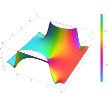
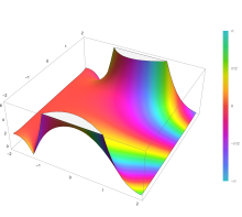
${displaystyle left({frac {c}{pi }}right)^{frac {1}{2}}int _{p}^{q}e^{-cx^{2}},mathrm {d} x={tfrac {1}{2}}left(operatorname {erf} left(q{sqrt {c}}right)-operatorname {erf} left(p{sqrt {c}}right)right).}$

Plot of the error function Erf(z) in the complex plane from -2-2i to 2+2i with colors created with Mathematica 13.1 function ComplexPlot3D

Applications[edit]

When the results of a series of measurements are described by a normal distribution with standard deviation σ and expected value 0, then erf (a/σ √2) is the probability that the error of a single measurement lies between −a and +a, for positive a. This is useful, for example, in determining the bit error rate of a digital communication system.

The error and complementary error functions occur, for example, in solutions of the heat equation when boundary conditions are given by the Heaviside step function.

The error function and its approximations can be used to estimate results that hold with high probability or with low probability. Given a random variable X ~ Norm[μ,σ] (a normal distribution with mean μ and standard deviation σ) and a constant L < μ:

${displaystyle {begin{aligned}Pr[Xleq L]&={frac {1}{2}}+{frac {1}{2}}operatorname {erf} {frac {L-mu }{{sqrt {2}}sigma }}\&approx Aexp left(-Bleft({frac {L-mu }{sigma }}right)^{2}right)end{aligned}}}$

where A and B are certain numeric constants. If L is sufficiently far from the mean, specifically μ − L ≥ σ√ln k, then:

${displaystyle Pr[Xleq L]leq Aexp(-Bln {k})={frac {A}{k^{B}}}}$

so the probability goes to 0 as k → ∞.

The probability for X being in the interval [L_a, L_b] can be derived as

${displaystyle {begin{aligned}Pr[L_{a}leq Xleq L_{b}]&=int _{L_{a}}^{L_{b}}{frac {1}{{sqrt {2pi }}sigma }}exp left(-{frac {(x-mu )^{2}}{2sigma ^{2}}}right),mathrm {d} x\&={frac {1}{2}}left(operatorname {erf} {frac {L_{b}-mu }{{sqrt {2}}sigma }}-operatorname {erf} {frac {L_{a}-mu }{{sqrt {2}}sigma }}right).end{aligned}}}$

Properties[edit]

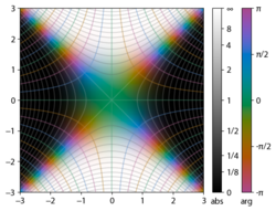
Integrand exp(−z²)

erf z

The property erf (−z) = −erf z means that the error function is an odd function. This directly results from the fact that the integrand e^−t² is an even function (the antiderivative of an even function which is zero at the origin is an odd function and vice versa).

Since the error function is an entire function which takes real numbers to real numbers, for any complex number z:

${displaystyle operatorname {erf} {overline {z}}={overline {operatorname {erf} z}}}$

where z is the complex conjugate of z.

The integrand f = exp(−z²) and f = erf z are shown in the complex z-plane in the figures at right with domain coloring.

The error function at +∞ is exactly 1 (see Gaussian integral). At the real axis, erf z approaches unity at z → +∞ and −1 at z → −∞. At the imaginary axis, it tends to ±i∞.

Taylor series[edit]

The error function is an entire function; it has no singularities (except that at infinity) and its Taylor expansion always converges, but is famously known «[…] for its bad convergence if x > 1.»^[4]

The defining integral cannot be evaluated in closed form in terms of elementary functions, but by expanding the integrand e^−z² into its Maclaurin series and integrating term by term, one obtains the error function’s Maclaurin series as:

${displaystyle {begin{aligned}operatorname {erf} z&={frac {2}{sqrt {pi }}}sum _{n=0}^{infty }{frac {(-1)^{n}z^{2n+1}}{n!(2n+1)}}\[6pt]&={frac {2}{sqrt {pi }}}left(z-{frac {z^{3}}{3}}+{frac {z^{5}}{10}}-{frac {z^{7}}{42}}+{frac {z^{9}}{216}}-cdots right)end{aligned}}}$

which holds for every complex number z. The denominator terms are sequence A007680 in the OEIS.

For iterative calculation of the above series, the following alternative formulation may be useful:

${displaystyle {begin{aligned}operatorname {erf} z&={frac {2}{sqrt {pi }}}sum _{n=0}^{infty }left(zprod _{k=1}^{n}{frac {-(2k-1)z^{2}}{k(2k+1)}}right)\[6pt]&={frac {2}{sqrt {pi }}}sum _{n=0}^{infty }{frac {z}{2n+1}}prod _{k=1}^{n}{frac {-z^{2}}{k}}end{aligned}}}$

because −(2k − 1)z²/k(2k + 1) expresses the multiplier to turn the kth term into the (k + 1)th term (considering z as the first term).

The imaginary error function has a very similar Maclaurin series, which is:

${displaystyle {begin{aligned}operatorname {erfi} z&={frac {2}{sqrt {pi }}}sum _{n=0}^{infty }{frac {z^{2n+1}}{n!(2n+1)}}\[6pt]&={frac {2}{sqrt {pi }}}left(z+{frac {z^{3}}{3}}+{frac {z^{5}}{10}}+{frac {z^{7}}{42}}+{frac {z^{9}}{216}}+cdots right)end{aligned}}}$

which holds for every complex number z.

Derivative and integral[edit]

The derivative of the error function follows immediately from its definition:

${displaystyle {frac {mathrm {d} }{mathrm {d} z}}operatorname {erf} z={frac {2}{sqrt {pi }}}e^{-z^{2}}.}$

From this, the derivative of the imaginary error function is also immediate:

${displaystyle {frac {d}{dz}}operatorname {erfi} z={frac {2}{sqrt {pi }}}e^{z^{2}}.}$

An antiderivative of the error function, obtainable by integration by parts, is

${displaystyle zoperatorname {erf} z+{frac {e^{-z^{2}}}{sqrt {pi }}}.}$

An antiderivative of the imaginary error function, also obtainable by integration by parts, is

${displaystyle zoperatorname {erfi} z-{frac {e^{z^{2}}}{sqrt {pi }}}.}$

Higher order derivatives are given by

${displaystyle operatorname {erf} ^{(k)}z={frac {2(-1)^{k-1}}{sqrt {pi }}}{mathit {H}}_{k-1}(z)e^{-z^{2}}={frac {2}{sqrt {pi }}}{frac {mathrm {d} ^{k-1}}{mathrm {d} z^{k-1}}}left(e^{-z^{2}}right),qquad k=1,2,dots }$

where H are the physicists’ Hermite polynomials.^[5]

Bürmann series[edit]

An expansion,^[6] which converges more rapidly for all real values of x than a Taylor expansion, is obtained by using Hans Heinrich Bürmann’s theorem:^[7]

${displaystyle {begin{aligned}operatorname {erf} x&={frac {2}{sqrt {pi }}}operatorname {sgn} xcdot {sqrt {1-e^{-x^{2}}}}left(1-{frac {1}{12}}left(1-e^{-x^{2}}right)-{frac {7}{480}}left(1-e^{-x^{2}}right)^{2}-{frac {5}{896}}left(1-e^{-x^{2}}right)^{3}-{frac {787}{276480}}left(1-e^{-x^{2}}right)^{4}-cdots right)\[10pt]&={frac {2}{sqrt {pi }}}operatorname {sgn} xcdot {sqrt {1-e^{-x^{2}}}}left({frac {sqrt {pi }}{2}}+sum _{k=1}^{infty }c_{k}e^{-kx^{2}}right).end{aligned}}}$

where sgn is the sign function. By keeping only the first two coefficients and choosing c₁ = 31/200 and c₂ = −341/8000, the resulting approximation shows its largest relative error at x = ±1.3796, where it is less than 0.0036127:

${displaystyle operatorname {erf} xapprox {frac {2}{sqrt {pi }}}operatorname {sgn} xcdot {sqrt {1-e^{-x^{2}}}}left({frac {sqrt {pi }}{2}}+{frac {31}{200}}e^{-x^{2}}-{frac {341}{8000}}e^{-2x^{2}}right).}$

Inverse functions[edit]

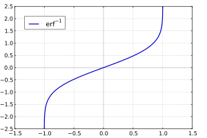
Given a complex number z, there is not a unique complex number w satisfying erf w = z, so a true inverse function would be multivalued. However, for −1 < x < 1, there is a unique real number denoted erf⁻¹ x satisfying

${displaystyle operatorname {erf} left(operatorname {erf} ^{-1}xright)=x.}$

The inverse error function is usually defined with domain (−1,1), and it is restricted to this domain in many computer algebra systems. However, it can be extended to the disk |z| < 1 of the complex plane, using the Maclaurin series

${displaystyle operatorname {erf} ^{-1}z=sum _{k=0}^{infty }{frac {c_{k}}{2k+1}}left({frac {sqrt {pi }}{2}}zright)^{2k+1},}$

where c₀ = 1 and

${displaystyle {begin{aligned}c_{k}&=sum _{m=0}^{k-1}{frac {c_{m}c_{k-1-m}}{(m+1)(2m+1)}}\&=left{1,1,{frac {7}{6}},{frac {127}{90}},{frac {4369}{2520}},{frac {34807}{16200}},ldots right}.end{aligned}}}$

So we have the series expansion (common factors have been canceled from numerators and denominators):

${displaystyle operatorname {erf} ^{-1}z={frac {sqrt {pi }}{2}}left(z+{frac {pi }{12}}z^{3}+{frac {7pi ^{2}}{480}}z^{5}+{frac {127pi ^{3}}{40320}}z^{7}+{frac {4369pi ^{4}}{5806080}}z^{9}+{frac {34807pi ^{5}}{182476800}}z^{11}+cdots right).}$

(After cancellation the numerator/denominator fractions are entries OEIS: A092676/OEIS: A092677 in the OEIS; without cancellation the numerator terms are given in entry OEIS: A002067.) The error function’s value at ±∞ is equal to ±1.

For |z| < 1, we have erf(erf⁻¹ z) = z.

The inverse complementary error function is defined as

${displaystyle operatorname {erfc} ^{-1}(1-z)=operatorname {erf} ^{-1}z.}$

For real x, there is a unique real number erfi⁻¹ x satisfying erfi(erfi⁻¹ x) = x. The inverse imaginary error function is defined as erfi⁻¹ x.^[8]

For any real x, Newton’s method can be used to compute erfi⁻¹ x, and for −1 ≤ x ≤ 1, the following Maclaurin series converges:

${displaystyle operatorname {erfi} ^{-1}z=sum _{k=0}^{infty }{frac {(-1)^{k}c_{k}}{2k+1}}left({frac {sqrt {pi }}{2}}zright)^{2k+1},}$

where c_k is defined as above.

Asymptotic expansion[edit]

A useful asymptotic expansion of the complementary error function (and therefore also of the error function) for large real x is

${displaystyle {begin{aligned}operatorname {erfc} x&={frac {e^{-x^{2}}}{x{sqrt {pi }}}}left(1+sum _{n=1}^{infty }(-1)^{n}{frac {1cdot 3cdot 5cdots (2n-1)}{left(2x^{2}right)^{n}}}right)\[6pt]&={frac {e^{-x^{2}}}{x{sqrt {pi }}}}sum _{n=0}^{infty }(-1)^{n}{frac {(2n-1)!!}{left(2x^{2}right)^{n}}},end{aligned}}}$

where (2n − 1)!! is the double factorial of (2n − 1), which is the product of all odd numbers up to (2n − 1). This series diverges for every finite x, and its meaning as asymptotic expansion is that for any integer N ≥ 1 one has

${displaystyle operatorname {erfc} x={frac {e^{-x^{2}}}{x{sqrt {pi }}}}sum _{n=0}^{N-1}(-1)^{n}{frac {(2n-1)!!}{left(2x^{2}right)^{n}}}+R_{N}(x)}$

where the remainder, in Landau notation, is

${displaystyle R_{N}(x)=Oleft(x^{-(1+2N)}e^{-x^{2}}right)}$

as x → ∞.

Indeed, the exact value of the remainder is

${displaystyle R_{N}(x):={frac {(-1)^{N}}{sqrt {pi }}}2^{1-2N}{frac {(2N)!}{N!}}int _{x}^{infty }t^{-2N}e^{-t^{2}},mathrm {d} t,}$

which follows easily by induction, writing

${displaystyle e^{-t^{2}}=-(2t)^{-1}left(e^{-t^{2}}right)'}$

and integrating by parts.

For large enough values of x, only the first few terms of this asymptotic expansion are needed to obtain a good approximation of erfc x (while for not too large values of x, the above Taylor expansion at 0 provides a very fast convergence).

Continued fraction expansion[edit]

A continued fraction expansion of the complementary error function is:^[9]

${displaystyle operatorname {erfc} z={frac {z}{sqrt {pi }}}e^{-z^{2}}{cfrac {1}{z^{2}+{cfrac {a_{1}}{1+{cfrac {a_{2}}{z^{2}+{cfrac {a_{3}}{1+dotsb }}}}}}}},qquad a_{m}={frac {m}{2}}.}$

Integral of error function with Gaussian density function[edit]

${displaystyle int _{-infty }^{infty }operatorname {erf} left(ax+bright){frac {1}{sqrt {2pi sigma ^{2}}}}exp left(-{frac {(x-mu )^{2}}{2sigma ^{2}}}right),mathrm {d} x=operatorname {erf} {frac {amu +b}{sqrt {1+2a^{2}sigma ^{2}}}},qquad a,b,mu ,sigma in mathbb {R} }$

which appears related to Ng and Geller, formula 13 in section 4.3^[10] with a change of variables.

Factorial series[edit]

The inverse factorial series:

${displaystyle {begin{aligned}operatorname {erfc} z&={frac {e^{-z^{2}}}{{sqrt {pi }},z}}sum _{n=0}^{infty }{frac {(-1)^{n}Q_{n}}{{(z^{2}+1)}^{bar {n}}}}\&={frac {e^{-z^{2}}}{{sqrt {pi }},z}}left(1-{frac {1}{2}}{frac {1}{(z^{2}+1)}}+{frac {1}{4}}{frac {1}{(z^{2}+1)(z^{2}+2)}}-cdots right)end{aligned}}}$

converges for Re(z²) > 0. Here

${displaystyle {begin{aligned}Q_{n}&{overset {text{def}}{{}={}}}{frac {1}{Gamma left({frac {1}{2}}right)}}int _{0}^{infty }tau (tau -1)cdots (tau -n+1)tau ^{-{frac {1}{2}}}e^{-tau },dtau \&=sum _{k=0}^{n}left({tfrac {1}{2}}right)^{bar {k}}s(n,k),end{aligned}}}$

zⁿ denotes the rising factorial, and s(n,k) denotes a signed Stirling number of the first kind.^[11]^[12]
There also exists a representation by an infinite sum containing the double factorial:

${displaystyle operatorname {erf} z={frac {2}{sqrt {pi }}}sum _{n=0}^{infty }{frac {(-2)^{n}(2n-1)!!}{(2n+1)!}}z^{2n+1}}$

Numerical approximations[edit]

Approximation with elementary functions[edit]

Abramowitz and Stegun give several approximations of varying accuracy (equations 7.1.25–28). This allows one to choose the fastest approximation suitable for a given application. In order of increasing accuracy, they are:

${displaystyle operatorname {erf} xapprox 1-{frac {1}{left(1+a_{1}x+a_{2}x^{2}+a_{3}x^{3}+a_{4}x^{4}right)^{4}}},qquad xgeq 0}$

(maximum error: 5×10⁻⁴)

where a₁ = 0.278393, a₂ = 0.230389, a₃ = 0.000972, a₄ = 0.078108

${displaystyle operatorname {erf} xapprox 1-left(a_{1}t+a_{2}t^{2}+a_{3}t^{3}right)e^{-x^{2}},quad t={frac {1}{1+px}},qquad xgeq 0}$

(maximum error: 2.5×10⁻⁵)

where p = 0.47047, a₁ = 0.3480242, a₂ = −0.0958798, a₃ = 0.7478556

${displaystyle operatorname {erf} xapprox 1-{frac {1}{left(1+a_{1}x+a_{2}x^{2}+cdots +a_{6}x^{6}right)^{16}}},qquad xgeq 0}$

(maximum error: 3×10⁻⁷)

where a₁ = 0.0705230784, a₂ = 0.0422820123, a₃ = 0.0092705272, a₄ = 0.0001520143, a₅ = 0.0002765672, a₆ = 0.0000430638

${displaystyle operatorname {erf} xapprox 1-left(a_{1}t+a_{2}t^{2}+cdots +a_{5}t^{5}right)e^{-x^{2}},quad t={frac {1}{1+px}}}$

(maximum error: 1.5×10⁻⁷)

where p = 0.3275911, a₁ = 0.254829592, a₂ = −0.284496736, a₃ = 1.421413741, a₄ = −1.453152027, a₅ = 1.061405429

All of these approximations are valid for x ≥ 0. To use these approximations for negative x, use the fact that erf x is an odd function, so erf x = −erf(−x).
Exponential bounds and a pure exponential approximation for the complementary error function are given by^[13]

${displaystyle {begin{aligned}operatorname {erfc} x&leq {tfrac {1}{2}}e^{-2x^{2}}+{tfrac {1}{2}}e^{-x^{2}}leq e^{-x^{2}},&quad x&>0\operatorname {erfc} x&approx {tfrac {1}{6}}e^{-x^{2}}+{tfrac {1}{2}}e^{-{frac {4}{3}}x^{2}},&quad x&>0.end{aligned}}}$
The above have been generalized to sums of N exponentials^[14] with increasing accuracy in terms of N so that erfc x can be accurately approximated or bounded by 2Q̃(√2x), where

${displaystyle {tilde {Q}}(x)=sum _{n=1}^{N}a_{n}e^{-b_{n}x^{2}}.}$

In particular, there is a systematic methodology to solve the numerical coefficients {(a_n,b_n)}^N
_{n = 1} that yield a minimax approximation or bound for the closely related Q-function: Q(x) ≈ Q̃(x), Q(x) ≤ Q̃(x), or Q(x) ≥ Q̃(x) for x ≥ 0. The coefficients {(a_n,b_n)}^N
_{n = 1} for many variations of the exponential approximations and bounds up to N = 25 have been released to open access as a comprehensive dataset.^[15]
A tight approximation of the complementary error function for x ∈ [0,∞) is given by Karagiannidis & Lioumpas (2007)^[16] who showed for the appropriate choice of parameters {A,B} that

${displaystyle operatorname {erfc} xapprox {frac {left(1-e^{-Ax}right)e^{-x^{2}}}{B{sqrt {pi }}x}}.}$

They determined {A,B} = {1.98,1.135}, which gave a good approximation for all x ≥ 0. Alternative coefficients are also available for tailoring accuracy for a specific application or transforming the expression into a tight bound.^[17]
A single-term lower bound is^[18]

${displaystyle operatorname {erfc} xgeq {sqrt {frac {2e}{pi }}}{frac {sqrt {beta -1}}{beta }}e^{-beta x^{2}},qquad xgeq 0,quad beta >1,}$

where the parameter β can be picked to minimize error on the desired interval of approximation.
Another approximation is given by Sergei Winitzki using his «global Padé approximations»:^[19]^[20]^: 2–3

${displaystyle operatorname {erf} xapprox operatorname {sgn} xcdot {sqrt {1-exp left(-x^{2}{frac {{frac {4}{pi }}+ax^{2}}{1+ax^{2}}}right)}}}$

where

${displaystyle a={frac {8(pi -3)}{3pi (4-pi )}}approx 0.140012.}$

This is designed to be very accurate in a neighborhood of 0 and a neighborhood of infinity, and the relative error is less than 0.00035 for all real x. Using the alternate value a ≈ 0.147 reduces the maximum relative error to about 0.00013.^[21]

This approximation can be inverted to obtain an approximation for the inverse error function:

${displaystyle operatorname {erf} ^{-1}xapprox operatorname {sgn} xcdot {sqrt {{sqrt {left({frac {2}{pi a}}+{frac {ln left(1-x^{2}right)}{2}}right)^{2}-{frac {ln left(1-x^{2}right)}{a}}}}-left({frac {2}{pi a}}+{frac {ln left(1-x^{2}right)}{2}}right)}}.}$
An approximation with a maximal error of 1.2×10⁻⁷ for any real argument is:^[22]

${displaystyle operatorname {erf} x={begin{cases}1-tau &xgeq 0\tau -1&x<0end{cases}}}$

with

${displaystyle {begin{aligned}tau &=tcdot exp left(-x^{2}-1.26551223+1.00002368t+0.37409196t^{2}+0.09678418t^{3}-0.18628806t^{4}right.\&left.qquad qquad qquad +0.27886807t^{5}-1.13520398t^{6}+1.48851587t^{7}-0.82215223t^{8}+0.17087277t^{9}right)end{aligned}}}$

and

${displaystyle t={frac {1}{1+{frac {1}{2}}|x|}}.}$

Table of values[edit]

x	erf x	1 − erf x
0	0	1
0.02	0.022564575	0.977435425
0.04	0.045111106	0.954888894
0.06	0.067621594	0.932378406
0.08	0.090078126	0.909921874
0.1	0.112462916	0.887537084
0.2	0.222702589	0.777297411
0.3	0.328626759	0.671373241
0.4	0.428392355	0.571607645
0.5	0.520499878	0.479500122
0.6	0.603856091	0.396143909
0.7	0.677801194	0.322198806
0.8	0.742100965	0.257899035
0.9	0.796908212	0.203091788
1	0.842700793	0.157299207
1.1	0.880205070	0.119794930
1.2	0.910313978	0.089686022
1.3	0.934007945	0.065992055
1.4	0.952285120	0.047714880
1.5	0.966105146	0.033894854
1.6	0.976348383	0.023651617
1.7	0.983790459	0.016209541
1.8	0.989090502	0.010909498
1.9	0.992790429	0.007209571
2	0.995322265	0.004677735
2.1	0.997020533	0.002979467
2.2	0.998137154	0.001862846
2.3	0.998856823	0.001143177
2.4	0.999311486	0.000688514
2.5	0.999593048	0.000406952
3	0.999977910	0.000022090
3.5	0.999999257	0.000000743

[edit]

Complementary error function[edit]

The complementary error function, denoted erfc, is defined as

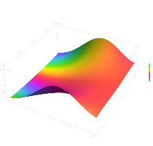
Plot of the complementary error function Erfc(z) in the complex plane from -2-2i to 2+2i with colors created with Mathematica 13.1 function ComplexPlot3D

${displaystyle {begin{aligned}operatorname {erfc} x&=1-operatorname {erf} x\[5pt]&={frac {2}{sqrt {pi }}}int _{x}^{infty }e^{-t^{2}},mathrm {d} t\[5pt]&=e^{-x^{2}}operatorname {erfcx} x,end{aligned}}}$

which also defines erfcx, the scaled complementary error function^[23] (which can be used instead of erfc to avoid arithmetic underflow^[23]^[24]). Another form of erfc x for x ≥ 0 is known as Craig’s formula, after its discoverer:^[25]

${displaystyle operatorname {erfc} (xmid xgeq 0)={frac {2}{pi }}int _{0}^{frac {pi }{2}}exp left(-{frac {x^{2}}{sin ^{2}theta }}right),mathrm {d} theta .}$

This expression is valid only for positive values of x, but it can be used in conjunction with erfc x = 2 − erfc(−x) to obtain erfc(x) for negative values. This form is advantageous in that the range of integration is fixed and finite. An extension of this expression for the erfc of the sum of two non-negative variables is as follows:^[26]

${displaystyle operatorname {erfc} (x+ymid x,ygeq 0)={frac {2}{pi }}int _{0}^{frac {pi }{2}}exp left(-{frac {x^{2}}{sin ^{2}theta }}-{frac {y^{2}}{cos ^{2}theta }}right),mathrm {d} theta .}$

Imaginary error function[edit]

The imaginary error function, denoted erfi, is defined as

Plot of the imaginary error function Erfi(z) in the complex plane from -2-2i to 2+2i with colors created with Mathematica 13.1 function ComplexPlot3D

${displaystyle {begin{aligned}operatorname {erfi} x&=-ioperatorname {erf} ix\[5pt]&={frac {2}{sqrt {pi }}}int _{0}^{x}e^{t^{2}},mathrm {d} t\[5pt]&={frac {2}{sqrt {pi }}}e^{x^{2}}D(x),end{aligned}}}$

where D(x) is the Dawson function (which can be used instead of erfi to avoid arithmetic overflow^[23]).

Despite the name «imaginary error function», erfi x is real when x is real.

When the error function is evaluated for arbitrary complex arguments z, the resulting complex error function is usually discussed in scaled form as the Faddeeva function:

$w(z)=e^{-z^{2}}operatorname {erfc} (-iz)=operatorname {erfcx} (-iz).$

Cumulative distribution function[edit]

The error function is essentially identical to the standard normal cumulative distribution function, denoted Φ, also named norm(x) by some software languages^{[citation needed]}, as they differ only by scaling and translation. Indeed,

the normal cumulative distribution function plotted in the complex plane

${displaystyle {begin{aligned}Phi (x)&={frac {1}{sqrt {2pi }}}int _{-infty }^{x}e^{tfrac {-t^{2}}{2}},mathrm {d} t\[6pt]&={frac {1}{2}}left(1+operatorname {erf} {frac {x}{sqrt {2}}}right)\[6pt]&={frac {1}{2}}operatorname {erfc} left(-{frac {x}{sqrt {2}}}right)end{aligned}}}$

or rearranged for erf and erfc:

${displaystyle {begin{aligned}operatorname {erf} (x)&=2Phi left(x{sqrt {2}}right)-1\[6pt]operatorname {erfc} (x)&=2Phi left(-x{sqrt {2}}right)\&=2left(1-Phi left(x{sqrt {2}}right)right).end{aligned}}}$

Consequently, the error function is also closely related to the Q-function, which is the tail probability of the standard normal distribution. The Q-function can be expressed in terms of the error function as

${displaystyle {begin{aligned}Q(x)&={frac {1}{2}}-{frac {1}{2}}operatorname {erf} {frac {x}{sqrt {2}}}\&={frac {1}{2}}operatorname {erfc} {frac {x}{sqrt {2}}}.end{aligned}}}$

The inverse of Φ is known as the normal quantile function, or probit function and may be expressed in terms of the inverse error function as

${displaystyle operatorname {probit} (p)=Phi ^{-1}(p)={sqrt {2}}operatorname {erf} ^{-1}(2p-1)=-{sqrt {2}}operatorname {erfc} ^{-1}(2p).}$

The standard normal cdf is used more often in probability and statistics, and the error function is used more often in other branches of mathematics.

The error function is a special case of the Mittag-Leffler function, and can also be expressed as a confluent hypergeometric function (Kummer’s function):

${displaystyle operatorname {erf} x={frac {2x}{sqrt {pi }}}Mleft({tfrac {1}{2}},{tfrac {3}{2}},-x^{2}right).}$

It has a simple expression in terms of the Fresnel integral.^{[further explanation needed]}

In terms of the regularized gamma function P and the incomplete gamma function,

${displaystyle operatorname {erf} x=operatorname {sgn} xcdot Pleft({tfrac {1}{2}},x^{2}right)={frac {operatorname {sgn} x}{sqrt {pi }}}gamma left({tfrac {1}{2}},x^{2}right).}$

sgn x is the sign function.

Generalized error functions[edit]

Graph of generalised error functions E_n(x):
grey curve: E₁(x) = 1 − e^−x/√π
red curve: E₂(x) = erf(x)
green curve: E₃(x)
blue curve: E₄(x)
gold curve: E₅(x).

Some authors discuss the more general functions:^{[citation needed]}

${displaystyle E_{n}(x)={frac {n!}{sqrt {pi }}}int _{0}^{x}e^{-t^{n}},mathrm {d} t={frac {n!}{sqrt {pi }}}sum _{p=0}^{infty }(-1)^{p}{frac {x^{np+1}}{(np+1)p!}}.}$

Notable cases are:

E₀(x) is a straight line through the origin: E₀(x) = x/e√π
E₂(x) is the error function, erf x.

After division by n!, all the E_n for odd n look similar (but not identical) to each other. Similarly, the E_n for even n look similar (but not identical) to each other after a simple division by n!. All generalised error functions for n > 0 look similar on the positive x side of the graph.

These generalised functions can equivalently be expressed for x > 0 using the gamma function and incomplete gamma function:

${displaystyle E_{n}(x)={frac {1}{sqrt {pi }}}Gamma (n)left(Gamma left({frac {1}{n}}right)-Gamma left({frac {1}{n}},x^{n}right)right),qquad x>0.}$

Therefore, we can define the error function in terms of the incomplete gamma function:

${displaystyle operatorname {erf} x=1-{frac {1}{sqrt {pi }}}Gamma left({tfrac {1}{2}},x^{2}right).}$

Iterated integrals of the complementary error function[edit]

The iterated integrals of the complementary error function are defined by^[27]

${displaystyle {begin{aligned}operatorname {i} ^{n}!operatorname {erfc} z&=int _{z}^{infty }operatorname {i} ^{n-1}!operatorname {erfc} zeta ,mathrm {d} zeta \[6pt]operatorname {i} ^{0}!operatorname {erfc} z&=operatorname {erfc} z\operatorname {i} ^{1}!operatorname {erfc} z&=operatorname {ierfc} z={frac {1}{sqrt {pi }}}e^{-z^{2}}-zoperatorname {erfc} z\operatorname {i} ^{2}!operatorname {erfc} z&={tfrac {1}{4}}left(operatorname {erfc} z-2zoperatorname {ierfc} zright)\end{aligned}}}$

The general recurrence formula is

${displaystyle 2ncdot operatorname {i} ^{n}!operatorname {erfc} z=operatorname {i} ^{n-2}!operatorname {erfc} z-2zcdot operatorname {i} ^{n-1}!operatorname {erfc} z}$

They have the power series

${displaystyle operatorname {i} ^{n}!operatorname {erfc} z=sum _{j=0}^{infty }{frac {(-z)^{j}}{2^{n-j}j!,Gamma left(1+{frac {n-j}{2}}right)}},}$

from which follow the symmetry properties

${displaystyle operatorname {i} ^{2m}!operatorname {erfc} (-z)=-operatorname {i} ^{2m}!operatorname {erfc} z+sum _{q=0}^{m}{frac {z^{2q}}{2^{2(m-q)-1}(2q)!(m-q)!}}}$

and

${displaystyle operatorname {i} ^{2m+1}!operatorname {erfc} (-z)=operatorname {i} ^{2m+1}!operatorname {erfc} z+sum _{q=0}^{m}{frac {z^{2q+1}}{2^{2(m-q)-1}(2q+1)!(m-q)!}}.}$

Implementations[edit]

As real function of a real argument[edit]

In Posix-compliant operating systems, the header math.h shall declare and the mathematical library libm shall provide the functions erf and erfc (double precision) as well as their single precision and extended precision counterparts erff, erfl and erfcf, erfcl.^[28]
The GNU Scientific Library provides erf, erfc, log(erf), and scaled error functions.^[29]

As complex function of a complex argument[edit]

libcerf, numeric C library for complex error functions, provides the complex functions cerf, cerfc, cerfcx and the real functions erfi, erfcx with approximately 13–14 digits precision, based on the Faddeeva function as implemented in the MIT Faddeeva Package

References[edit]

^ Andrews, Larry C. (1998). Special functions of mathematics for engineers. SPIE Press. p. 110. ISBN 9780819426161.
^ Glaisher, James Whitbread Lee (July 1871). «On a class of definite integrals». London, Edinburgh, and Dublin Philosophical Magazine and Journal of Science. 4. 42 (277): 294–302. doi:10.1080/14786447108640568. Retrieved 6 December 2017.
^ Glaisher, James Whitbread Lee (September 1871). «On a class of definite integrals. Part II». London, Edinburgh, and Dublin Philosophical Magazine and Journal of Science. 4. 42 (279): 421–436. doi:10.1080/14786447108640600. Retrieved 6 December 2017.
^ «A007680 – OEIS». oeis.org. Retrieved 2 April 2020.
^ Weisstein, Eric W. «Erf». MathWorld.
^ Schöpf, H. M.; Supancic, P. H. (2014). «On Bürmann’s Theorem and Its Application to Problems of Linear and Nonlinear Heat Transfer and Diffusion». The Mathematica Journal. 16. doi:10.3888/tmj.16-11.
^ Weisstein, Eric W. «Bürmann’s Theorem». MathWorld.
^ Bergsma, Wicher (2006). «On a new correlation coefficient, its orthogonal decomposition and associated tests of independence». arXiv:math/0604627.
^ Cuyt, Annie A. M.; Petersen, Vigdis B.; Verdonk, Brigitte; Waadeland, Haakon; Jones, William B. (2008). Handbook of Continued Fractions for Special Functions. Springer-Verlag. ISBN 978-1-4020-6948-2.
^ Ng, Edward W.; Geller, Murray (January 1969). «A table of integrals of the Error functions». Journal of Research of the National Bureau of Standards Section B. 73B (1): 1. doi:10.6028/jres.073B.001.
^ Schlömilch, Oskar Xavier (1859). «Ueber facultätenreihen». Zeitschrift für Mathematik und Physik (in German). 4: 390–415. Retrieved 4 December 2017.
^ Nielson, Niels (1906). Handbuch der Theorie der Gammafunktion (in German). Leipzig: B. G. Teubner. p. 283 Eq. 3. Retrieved 4 December 2017.
^ Chiani, M.; Dardari, D.; Simon, M.K. (2003). «New Exponential Bounds and Approximations for the Computation of Error Probability in Fading Channels» (PDF). IEEE Transactions on Wireless Communications. 2 (4): 840–845. CiteSeerX 10.1.1.190.6761. doi:10.1109/TWC.2003.814350.
^ Tanash, I.M.; Riihonen, T. (2020). «Global minimax approximations and bounds for the Gaussian Q-function by sums of exponentials». IEEE Transactions on Communications. 68 (10): 6514–6524. arXiv:2007.06939. doi:10.1109/TCOMM.2020.3006902. S2CID 220514754.
^ Tanash, I.M.; Riihonen, T. (2020). «Coefficients for Global Minimax Approximations and Bounds for the Gaussian Q-Function by Sums of Exponentials [Data set]». Zenodo. doi:10.5281/zenodo.4112978.
^ Karagiannidis, G. K.; Lioumpas, A. S. (2007). «An improved approximation for the Gaussian Q-function» (PDF). IEEE Communications Letters. 11 (8): 644–646. doi:10.1109/LCOMM.2007.070470. S2CID 4043576.
^ Tanash, I.M.; Riihonen, T. (2021). «Improved coefficients for the Karagiannidis–Lioumpas approximations and bounds to the Gaussian Q-function». IEEE Communications Letters. 25 (5): 1468–1471. arXiv:2101.07631. doi:10.1109/LCOMM.2021.3052257. S2CID 231639206.
^ Chang, Seok-Ho; Cosman, Pamela C.; Milstein, Laurence B. (November 2011). «Chernoff-Type Bounds for the Gaussian Error Function». IEEE Transactions on Communications. 59 (11): 2939–2944. doi:10.1109/TCOMM.2011.072011.100049. S2CID 13636638.
^ Winitzki, Sergei (2003). «Uniform approximations for transcendental functions». Computational Science and Its Applications – ICCSA 2003. Lecture Notes in Computer Science. Vol. 2667. Springer, Berlin. pp. 780–789. doi:10.1007/3-540-44839-X_82. ISBN 978-3-540-40155-1.
^ Zeng, Caibin; Chen, Yang Cuan (2015). «Global Padé approximations of the generalized Mittag-Leffler function and its inverse». Fractional Calculus and Applied Analysis. 18 (6): 1492–1506. arXiv:1310.5592. doi:10.1515/fca-2015-0086. S2CID 118148950. Indeed, Winitzki [32] provided the so-called global Padé approximation
^ Winitzki, Sergei (6 February 2008). «A handy approximation for the error function and its inverse».
^ Numerical Recipes in Fortran 77: The Art of Scientific Computing (ISBN 0-521-43064-X), 1992, page 214, Cambridge University Press.
^ ^a ^b ^c Cody, W. J. (March 1993), «Algorithm 715: SPECFUN—A portable FORTRAN package of special function routines and test drivers» (PDF), ACM Trans. Math. Softw., 19 (1): 22–32, CiteSeerX 10.1.1.643.4394, doi:10.1145/151271.151273, S2CID 5621105
^ Zaghloul, M. R. (1 March 2007), «On the calculation of the Voigt line profile: a single proper integral with a damped sine integrand», Monthly Notices of the Royal Astronomical Society, 375 (3): 1043–1048, Bibcode:2007MNRAS.375.1043Z, doi:10.1111/j.1365-2966.2006.11377.x
^ John W. Craig, A new, simple and exact result for calculating the probability of error for two-dimensional signal constellations Archived 3 April 2012 at the Wayback Machine, Proceedings of the 1991 IEEE Military Communication Conference, vol. 2, pp. 571–575.
^ Behnad, Aydin (2020). «A Novel Extension to Craig’s Q-Function Formula and Its Application in Dual-Branch EGC Performance Analysis». IEEE Transactions on Communications. 68 (7): 4117–4125. doi:10.1109/TCOMM.2020.2986209. S2CID 216500014.
^ Carslaw, H. S.; Jaeger, J. C. (1959), Conduction of Heat in Solids (2nd ed.), Oxford University Press, ISBN 978-0-19-853368-9, p 484
^ https://pubs.opengroup.org/onlinepubs/9699919799/basedefs/math.h.html
^ «Special Functions – GSL 2.7 documentation».

External links[edit]

A Table of Integrals of the Error Functions

Источник

Error function
Plot of the error function
General information
General definition	${displaystyle operatorname {erf} z={frac {2}{sqrt {pi }}}int _{0}^{z}e^{-t^{2}},mathrm {d} t}$
Fields of application	Probability, thermodynamics
Domain, Codomain and Image
Domain	$mathbb {C}$
Image	${displaystyle left(-1,1right)}$
Basic features
Parity	Odd
Specific features
Root	0
Derivative	${displaystyle {frac {mathrm {d} }{mathrm {d} z}}operatorname {erf} z={frac {2}{sqrt {pi }}}e^{-z^{2}}}$
Antiderivative	${displaystyle int operatorname {erf} z,dz=zoperatorname {erf} z+{frac {e^{-z^{2}}}{sqrt {pi }}}+C}$
Series definition
Taylor series	${displaystyle operatorname {erf} z={frac {2}{sqrt {pi }}}sum _{n=0}^{infty }{frac {z}{2n+1}}prod _{k=1}^{n}{frac {-z^{2}}{k}}}$