Представление результатов исследования
В научных публикациях важно представление результатов исследования. Очень часто окончательный результат приводится в следующем виде: M±m, где M – среднее арифметическое, m –ошибка среднего арифметического. Например, 163,7±0,9 см.
Прежде чем разбираться в правилах представления результатов исследования, давайте точно усвоим, что же такое ошибка среднего арифметического.
Ошибка среднего арифметического
Среднее арифметическое, вычисленное на основе выборочных данных (выборочное среднее), как правило, не совпадает с генеральным средним (средним арифметическим генеральной совокупности). Экспериментально проверить это утверждение невозможно, потому что нам неизвестно генеральное среднее. Но если из одной и той же генеральной совокупности брать повторные выборки и вычислять среднее арифметическое, то окажется, что для разных выборок среднее арифметическое будет разным.
Чтобы оценить, насколько выборочное среднее арифметическое отличается от генерального среднего, вычисляется ошибка среднего арифметического или ошибка репрезентативности.
Ошибка среднего арифметического обозначается как m или 
Ошибка среднего арифметического рассчитывается по формуле:
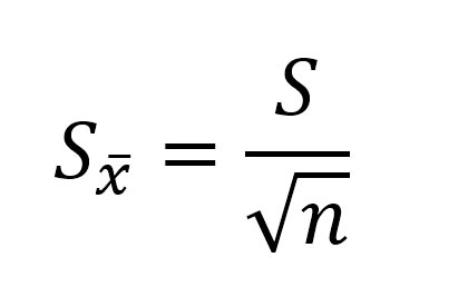
где: S — стандартное отклонение, n – объем выборки; Например, если стандартное отклонение равно S=5 см, объем выборки n=36 человек, то ошибка среднего арифметического равна: m=5/6 = 0,833.
Ошибка среднего арифметического показывает, какая ошибка в среднем допускается, если использовать вместо генерального среднего выборочное среднее.
Так как при небольшом объеме выборки истинное значение генерального среднего не может быть определено сколь угодно точно, поэтому при вычислении выборочного среднего арифметического нет смысла оставлять большое число значащих цифр.
Правила записи результатов исследования
- В записи ошибки среднего арифметического оставляем две значащие цифры, если первые цифры в ошибке «1» или «2».
- В остальных случаях в записи ошибки среднего арифметического оставляем одну значащую цифру.
- В записи среднего арифметического положение последней значащей цифры должно соответствовать положению первой значащей цифры в записи ошибки среднего арифметического.
Представление результатов научных исследований
В своей статье «Осторожно, статистика!», опубликованной в 1989 году В.М. Зациорский указал, какие числовые характеристики должны быть представлены в публикации, чтобы она имела научную ценность. Он писал, что исследователь «…должен назвать: 1) среднюю величину (или другой так называемый показатель положения); 2) среднее квадратическое отклонение (или другой показатель рассеяния) и 3) число испытуемых. Без них его публикация научной ценности иметь не будет “с. 52
В научных публикациях в области физической культуры и спорта очень часто окончательный результат приводится в виде: (М±m) (табл.1).
Таблица 1 — Изменение механических свойств латеральной широкой мышцы бедра под воздействием физической нагрузки (n=34)
| Эффективный модуль
упругости (Е), кПа |
Эффективный модуль
вязкости (V), Па с |
|||
| Этап
эксперимента |
Рассл. | Напряж. | Рассл. | Напряж. |
| До ФН | 7,0±0,3 | 17,1±1,4 | 29,7±1,7 | 46±4 |
| После ФН | 7,7±0,3 | 18,7±1,4 | 30,9±2,0 | 53±6 |
Литература
- Высшая математика и математическая статистика: учебное пособие для вузов / Под общ. ред. Г. И. Попова. – М. Физическая культура, 2007.– 368 с.
- Гласс Дж., Стэнли Дж. Статистические методы в педагогике и психологии. М.: Прогресс. 1976.- 495 с.
- Зациорский В.М. Осторожно — статистика! // Теория и практика физической культуры, 1989.- №2.
- Катранов А.Г. Компьютерная обработка данных экспериментальных исследований: Учебное пособие/ А. Г. Катранов, А. В. Самсонова; СПб ГУФК им. П.Ф. Лесгафта. – СПб.: изд-во СПб ГУФК им. П.Ф. Лесгафта, 2005. – 131 с.
- Основы математической статистики: Учебное пособие для ин-тов физ. культ / Под ред. В.С. Иванова.– М.: Физкультура и спорт, 1990. 176 с.
Чтобы
судить о том, насколько точно проведенные
измерения отражают состав генеральной
совокупности, необходимо вычислить
стандартную ошибку средней арифметической
выборочной совокупности.
Стандартная
ошибка средней арифметической
характеризует степень отклонения
выборочной средней арифметической от
средней арифметической генеральной
совокупности.
Стандартная
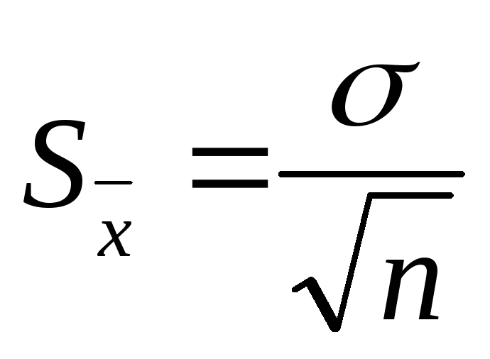
ошибка средней арифметической вычисляется
по формуле:
 ,
,
где
– стандартное отклонение результатов
измерений, n
– объем выборки.
Зачастую
мы имеем дело с одной случайной выборкой
и с одной полученной при ее обработке
выборочной средней. Задача заключается
в суждении о величине неизвестной
генеральной средней по полученной
неточной величине случайной выборочной
средней.
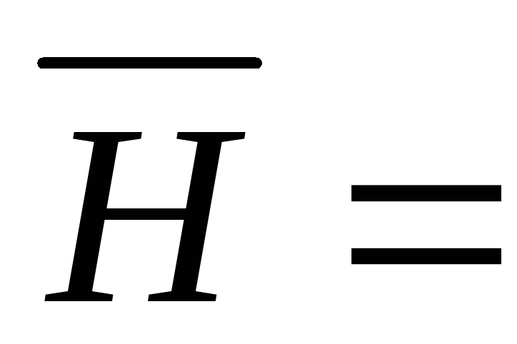
Вычислим
среднюю ошибку найденного выборочного
среднего значения роста:
 195
195
см; σ = 8,8 см;
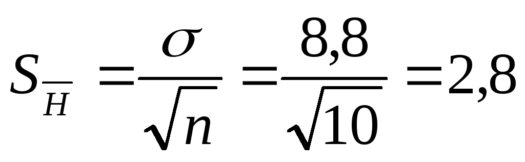 см.
см.
2,8 см
составляют не максимальную, а среднюю
возможную ошибку среднего. Отдельные
выборочные средние могут отклоняться
от генеральной как больше, так и меньше,
чем на 2,8 см.
Каковы
же пределы возможных ошибок случайной
выборки, какова ее максимальная ошибка?
Величина максимальной ошибки зависит
от величины средней ошибки и вычисляется
по формуле
 .
.
При
объеме выборки n
= 10:
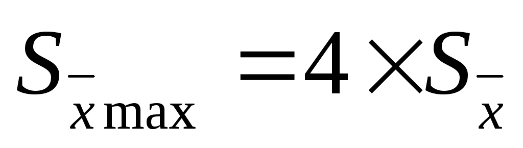 .
.
Все
случайные выборочные средние, которые
могут быть получены в подобных опытах
(в том числе и фактически полученная
выборочная средняя
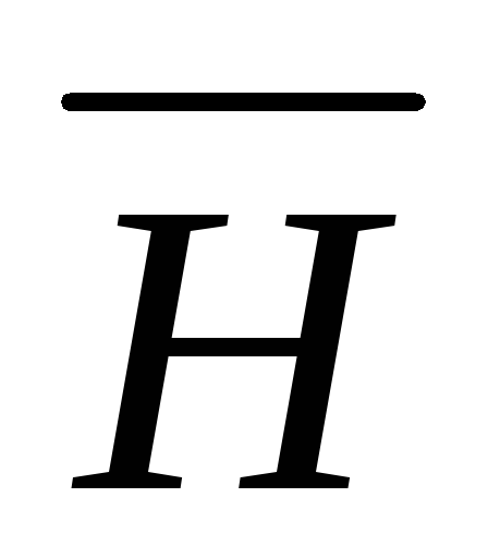 = 195 см), при своем варьировании около
неизвестного генерального среднего в
подавляющем количестве группируются
около него так, что лишь ничтожный
процент их отклоняется от генеральной
средней более, чем на величину максимальной
ошибки.
Другими
словами, генеральная средняя определяется
как
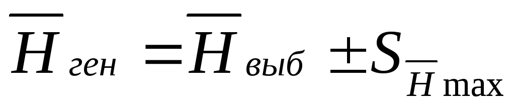 .
.
Эти пределы
колебаний значительно сужаются, если
средняя ошибка уменьшается благодаря
увеличению численности выборки.
Искомая
генеральная средняя лежит между
 и
и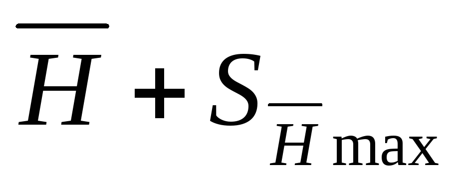 .
.
Таким образом, при высокой точности
выполнения эксперимента и достаточно
большом числе измерений можно определить
среднюю арифметическую бесконечно
большого числа экспериментов.
До сих
пор мы определяли максимальную ошибку
выборочной средней, исходя из того, что
все остальные показатели известны. Если
же мы хотим достичь определенной
точности, определенного приближения к
генеральной средней, в этом случае
встает вопрос о численности выборки (о
том, сколько измерений, опытов необходимо
провести).
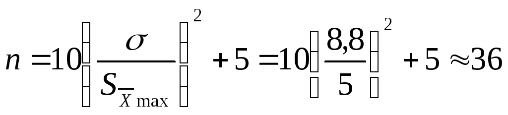
Допустим, что
максимальная ошибка должна быть равна
5 см. Сколько человек надо обследовать
(измерить) в нашем случае?
 .
.
Следовательно,
мы должны провести измерения роста у
36 баскетболистов высокого класса.
10. Достоверность различий
Следующим
важным вопросом практически для каждого
экспериментатора является умение
доказать достоверность различий между
двумя рядами признаков.
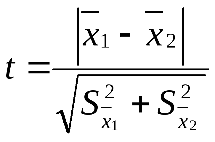
Проверку
достоверности различия двух рядов
измерений производят путем вычисления
критерия достоверности различия – t:
 ,
,
где
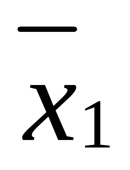 – средняя одной выборки;
 – средняя другой выборки;
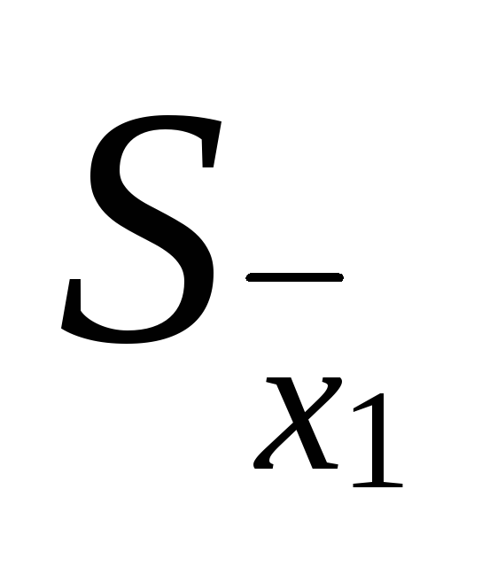 – средняя ошибка первой выборки;
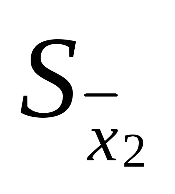 – второй выборки. Если t < 2, то различие
между двумя выборками считается
недостоверным, если t
2, то различие между двумя выборками
достоверно на 95%.
Соседние файлы в предмете [НЕСОРТИРОВАННОЕ]
- #
- #
- #
- #
- #
- #
- #
- #
- #
- #
- #
Содержание
- Расчет ошибки средней арифметической
- Способ 1: расчет с помощью комбинации функций
- Способ 2: применение инструмента «Описательная статистика»
- Вопросы и ответы

Стандартная ошибка или, как часто называют, ошибка средней арифметической, является одним из важных статистических показателей. С помощью данного показателя можно определить неоднородность выборки. Он также довольно важен при прогнозировании. Давайте узнаем, какими способами можно рассчитать величину стандартной ошибки с помощью инструментов Microsoft Excel.
Расчет ошибки средней арифметической
Одним из показателей, которые характеризуют цельность и однородность выборки, является стандартная ошибка. Эта величина представляет собой корень квадратный из дисперсии. Сама дисперсия является средним квадратном от средней арифметической. Средняя арифметическая вычисляется делением суммарной величины объектов выборки на их общее количество.
В Экселе существуют два способа вычисления стандартной ошибки: используя набор функций и при помощи инструментов Пакета анализа. Давайте подробно рассмотрим каждый из этих вариантов.
Способ 1: расчет с помощью комбинации функций
Прежде всего, давайте составим алгоритм действий на конкретном примере по расчету ошибки средней арифметической, используя для этих целей комбинацию функций. Для выполнения задачи нам понадобятся операторы СТАНДОТКЛОН.В, КОРЕНЬ и СЧЁТ.
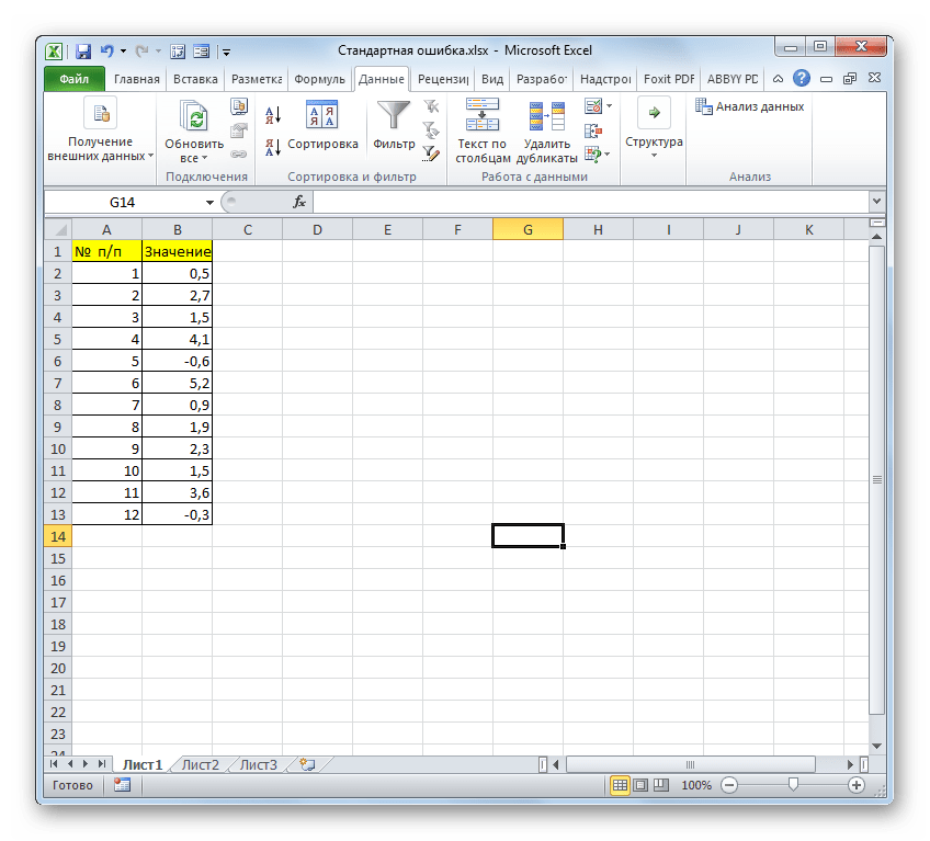
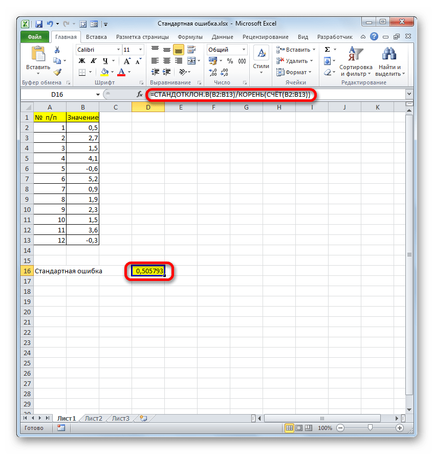
Для примера нами будет использована выборка из двенадцати чисел, представленных в таблице.
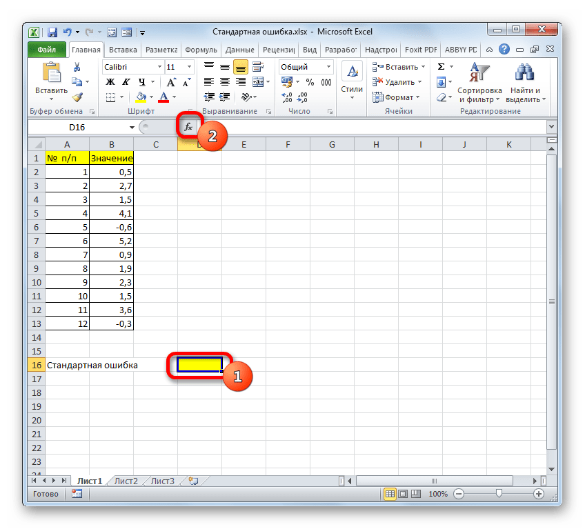
- Выделяем ячейку, в которой будет выводиться итоговое значение стандартной ошибки, и клацаем по иконке «Вставить функцию».
- Открывается Мастер функций. Производим перемещение в блок «Статистические». В представленном перечне наименований выбираем название «СТАНДОТКЛОН.В».
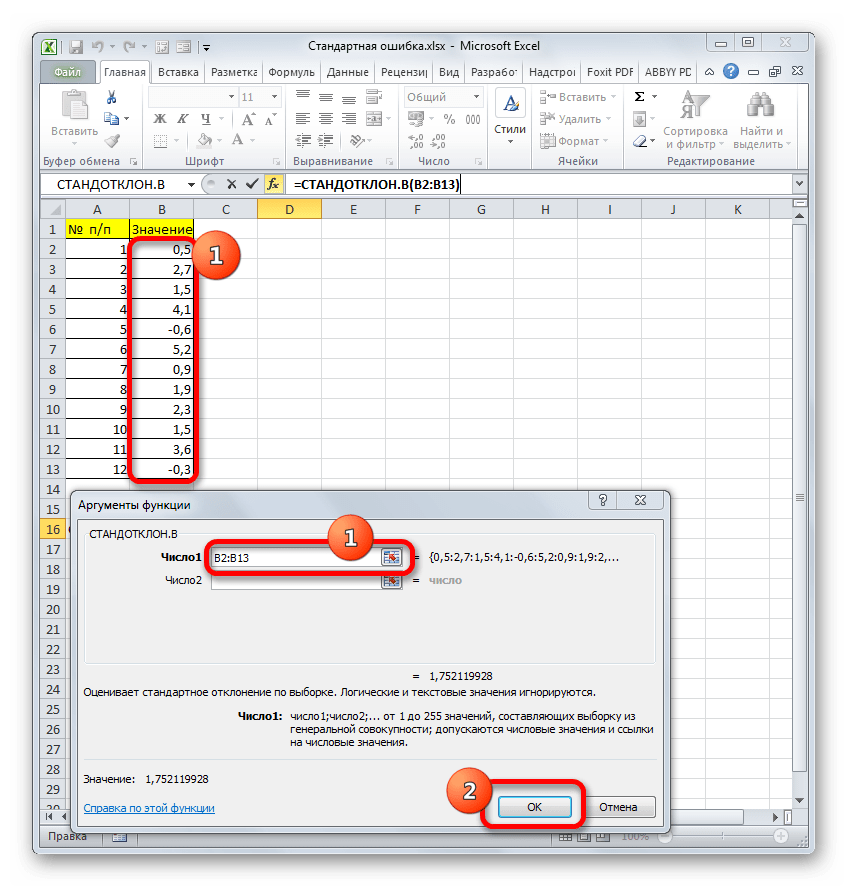
- Запускается окно аргументов вышеуказанного оператора. СТАНДОТКЛОН.В предназначен для оценивания стандартного отклонения при выборке. Данный оператор имеет следующий синтаксис:
=СТАНДОТКЛОН.В(число1;число2;…)«Число1» и последующие аргументы являются числовыми значениями или ссылками на ячейки и диапазоны листа, в которых они расположены. Всего может насчитываться до 255 аргументов этого типа. Обязательным является только первый аргумент.
Итак, устанавливаем курсор в поле «Число1». Далее, обязательно произведя зажим левой кнопки мыши, выделяем курсором весь диапазон выборки на листе. Координаты данного массива тут же отображаются в поле окна. После этого клацаем по кнопке «OK».
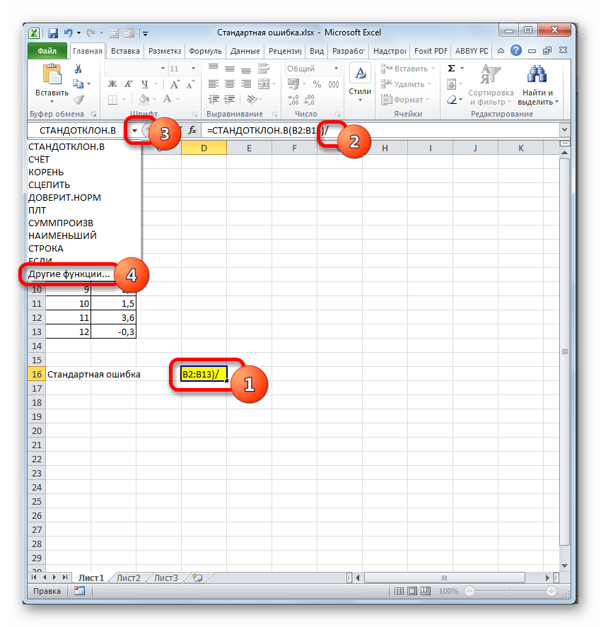
- В ячейку на листе выводится результат расчета оператора СТАНДОТКЛОН.В. Но это ещё не ошибка средней арифметической. Для того, чтобы получить искомое значение, нужно стандартное отклонение разделить на квадратный корень от количества элементов выборки. Для того, чтобы продолжить вычисления, выделяем ячейку, содержащую функцию СТАНДОТКЛОН.В. После этого устанавливаем курсор в строку формул и дописываем после уже существующего выражения знак деления (/). Вслед за этим клацаем по пиктограмме перевернутого вниз углом треугольника, которая располагается слева от строки формул. Открывается список недавно использованных функций. Если вы в нем найдете наименование оператора «КОРЕНЬ», то переходите по данному наименованию. В обратном случае жмите по пункту «Другие функции…».
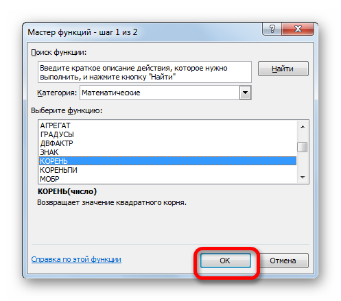
- Снова происходит запуск Мастера функций. На этот раз нам следует посетить категорию «Математические». В представленном перечне выделяем название «КОРЕНЬ» и жмем на кнопку «OK».
- Открывается окно аргументов функции КОРЕНЬ. Единственной задачей данного оператора является вычисление квадратного корня из заданного числа. Его синтаксис предельно простой:
=КОРЕНЬ(число)
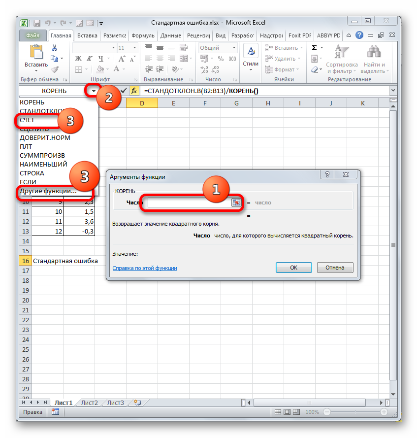
Как видим, функция имеет всего один аргумент «Число». Он может быть представлен числовым значением, ссылкой на ячейку, в которой оно содержится или другой функцией, вычисляющей это число. Последний вариант как раз и будет представлен в нашем примере.
Устанавливаем курсор в поле «Число» и кликаем по знакомому нам треугольнику, который вызывает список последних использованных функций. Ищем в нем наименование «СЧЁТ». Если находим, то кликаем по нему. В обратном случае, опять же, переходим по наименованию «Другие функции…».
- В раскрывшемся окне Мастера функций производим перемещение в группу «Статистические». Там выделяем наименование «СЧЁТ» и выполняем клик по кнопке «OK».
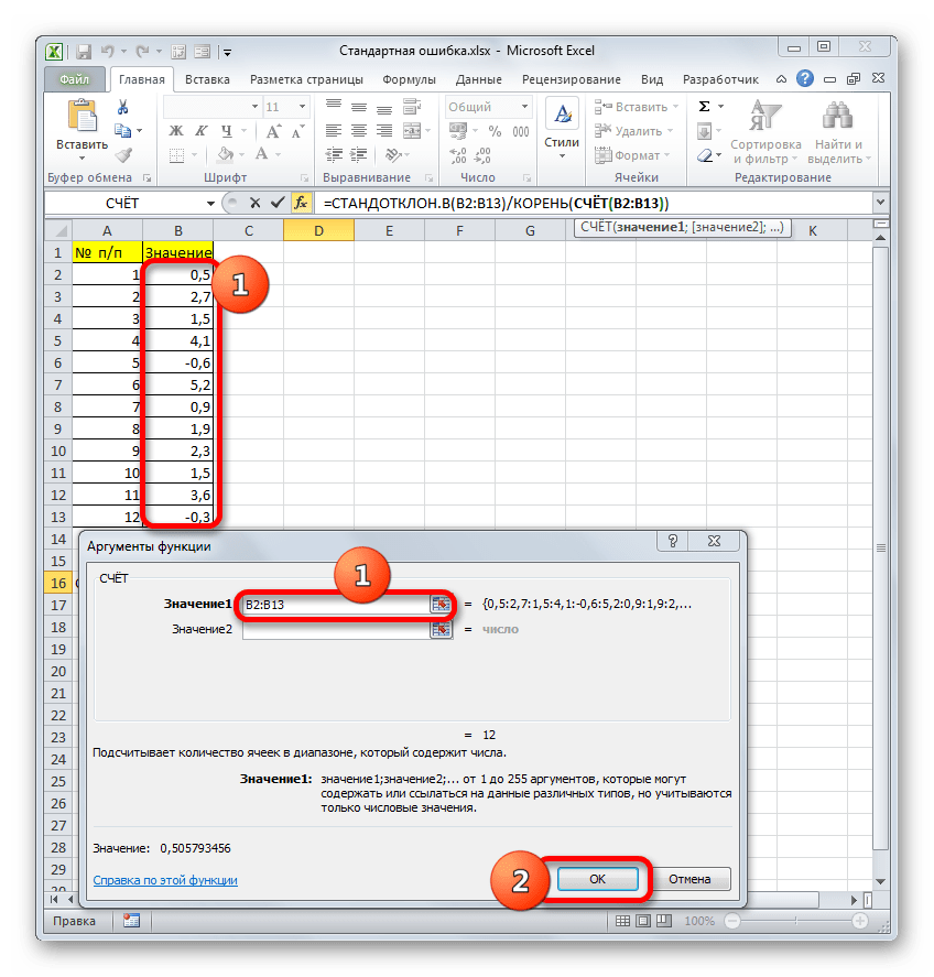
- Запускается окно аргументов функции СЧЁТ. Указанный оператор предназначен для вычисления количества ячеек, которые заполнены числовыми значениями. В нашем случае он будет подсчитывать количество элементов выборки и сообщать результат «материнскому» оператору КОРЕНЬ. Синтаксис функции следующий:
=СЧЁТ(значение1;значение2;…)В качестве аргументов «Значение», которых может насчитываться до 255 штук, выступают ссылки на диапазоны ячеек. Ставим курсор в поле «Значение1», зажимаем левую кнопку мыши и выделяем весь диапазон выборки. После того, как его координаты отобразились в поле, жмем на кнопку «OK».
- После выполнения последнего действия будет не только рассчитано количество ячеек заполненных числами, но и вычислена ошибка средней арифметической, так как это был последний штрих в работе над данной формулой. Величина стандартной ошибки выведена в ту ячейку, где размещена сложная формула, общий вид которой в нашем случае следующий:
=СТАНДОТКЛОН.В(B2:B13)/КОРЕНЬ(СЧЁТ(B2:B13))Результат вычисления ошибки средней арифметической составил 0,505793. Запомним это число и сравним с тем, которое получим при решении поставленной задачи следующим способом.


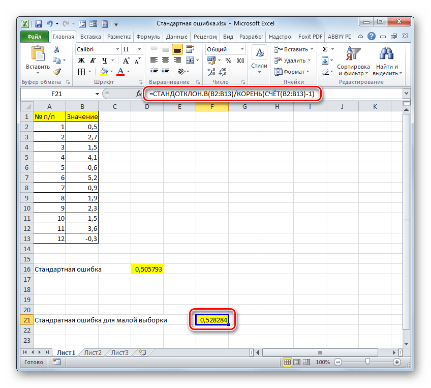
Но дело в том, что для малых выборок (до 30 единиц) для большей точности лучше применять немного измененную формулу. В ней величина стандартного отклонения делится не на квадратный корень от количества элементов выборки, а на квадратный корень от количества элементов выборки минус один. Таким образом, с учетом нюансов малой выборки наша формула приобретет следующий вид:
=СТАНДОТКЛОН.В(B2:B13)/КОРЕНЬ(СЧЁТ(B2:B13)-1)
Урок: Статистические функции в Экселе
Способ 2: применение инструмента «Описательная статистика»
Вторым вариантом, с помощью которого можно вычислить стандартную ошибку в Экселе, является применение инструмента «Описательная статистика», входящего в набор инструментов «Анализ данных» («Пакет анализа»). «Описательная статистика» проводит комплексный анализ выборки по различным критериям. Одним из них как раз и является нахождение ошибки средней арифметической.
Но чтобы воспользоваться данной возможностью, нужно сразу активировать «Пакет анализа», так как по умолчанию в Экселе он отключен.
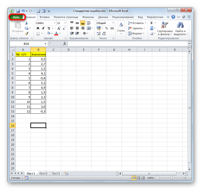
- После того, как открыт документ с выборкой, переходим во вкладку «Файл».
- Далее, воспользовавшись левым вертикальным меню, перемещаемся через его пункт в раздел «Параметры».
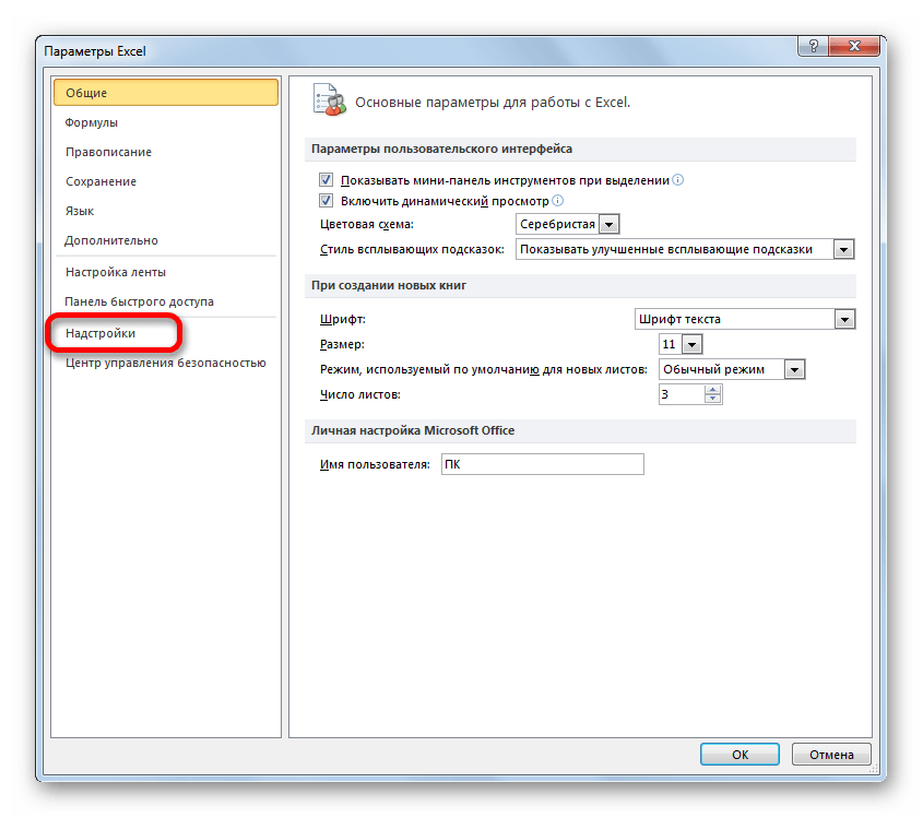
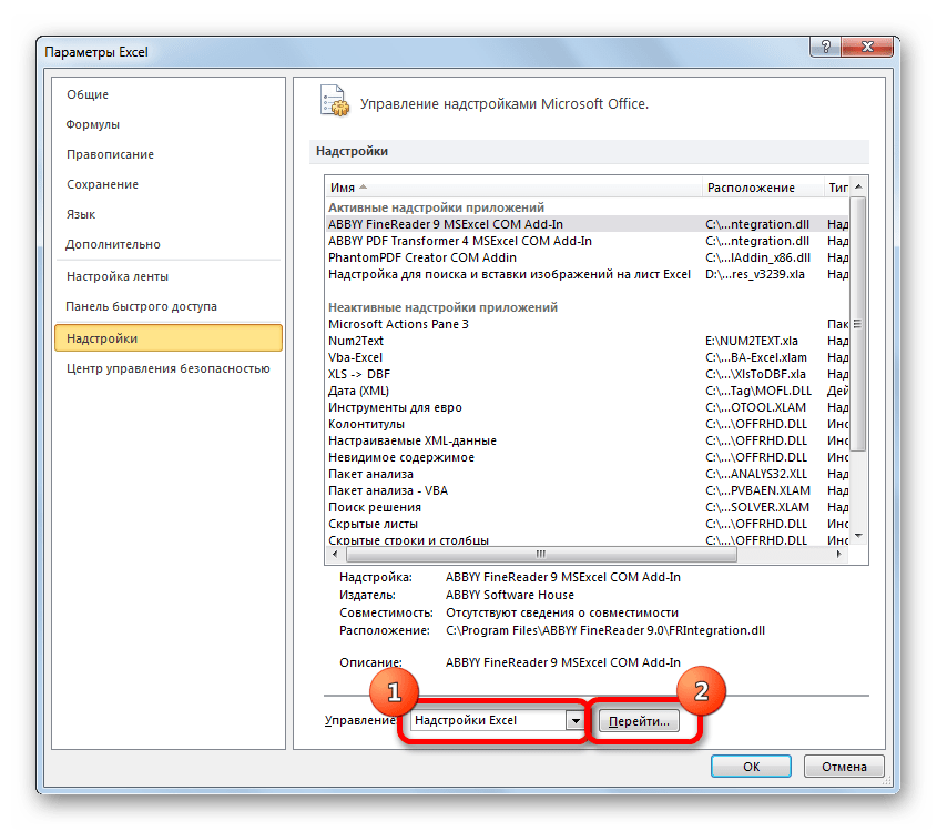
- Запускается окно параметров Эксель. В левой части данного окна размещено меню, через которое перемещаемся в подраздел «Надстройки».
- В самой нижней части появившегося окна расположено поле «Управление». Выставляем в нем параметр «Надстройки Excel» и жмем на кнопку «Перейти…» справа от него.
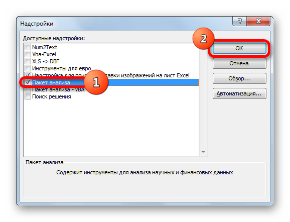
- Запускается окно надстроек с перечнем доступных скриптов. Отмечаем галочкой наименование «Пакет анализа» и щелкаем по кнопке «OK» в правой части окошка.
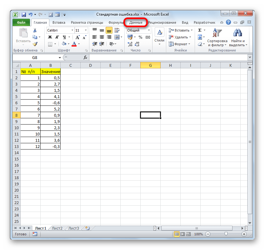
- После выполнения последнего действия на ленте появится новая группа инструментов, которая имеет наименование «Анализ». Чтобы перейти к ней, щелкаем по названию вкладки «Данные».
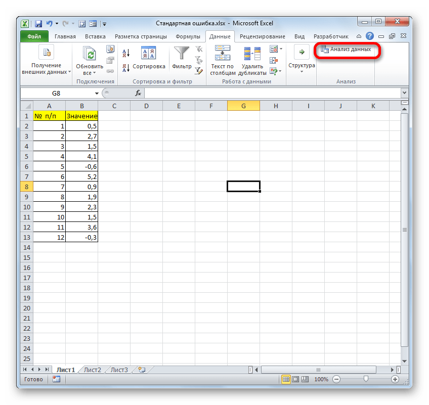
- После перехода жмем на кнопку «Анализ данных» в блоке инструментов «Анализ», который расположен в самом конце ленты.
- Запускается окошко выбора инструмента анализа. Выделяем наименование «Описательная статистика» и жмем на кнопку «OK» справа.
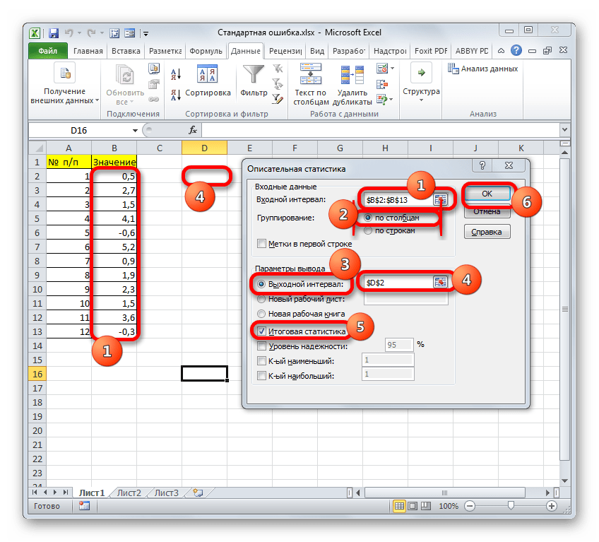
- Запускается окно настроек инструмента комплексного статистического анализа «Описательная статистика».
В поле «Входной интервал» необходимо указать диапазон ячеек таблицы, в которых находится анализируемая выборка. Вручную это делать неудобно, хотя и можно, поэтому ставим курсор в указанное поле и при зажатой левой кнопке мыши выделяем соответствующий массив данных на листе. Его координаты тут же отобразятся в поле окна.
В блоке «Группирование» оставляем настройки по умолчанию. То есть, переключатель должен стоять около пункта «По столбцам». Если это не так, то его следует переставить.
Галочку «Метки в первой строке» можно не устанавливать. Для решения нашего вопроса это не важно.
Далее переходим к блоку настроек «Параметры вывода». Здесь следует указать, куда именно будет выводиться результат расчета инструмента «Описательная статистика»:
- На новый лист;
- В новую книгу (другой файл);
- В указанный диапазон текущего листа.
Давайте выберем последний из этих вариантов. Для этого переставляем переключатель в позицию «Выходной интервал» и устанавливаем курсор в поле напротив данного параметра. После этого клацаем на листе по ячейке, которая станет верхним левым элементом массива вывода данных. Её координаты должны отобразиться в поле, в котором мы до этого устанавливали курсор.
Далее следует блок настроек определяющий, какие именно данные нужно вводить:
- Итоговая статистика;
- К-ый наибольший;
- К-ый наименьший;
- Уровень надежности.
Для определения стандартной ошибки обязательно нужно установить галочку около параметра «Итоговая статистика». Напротив остальных пунктов выставляем галочки на свое усмотрение. На решение нашей основной задачи это никак не повлияет.
После того, как все настройки в окне «Описательная статистика» установлены, щелкаем по кнопке «OK» в его правой части.
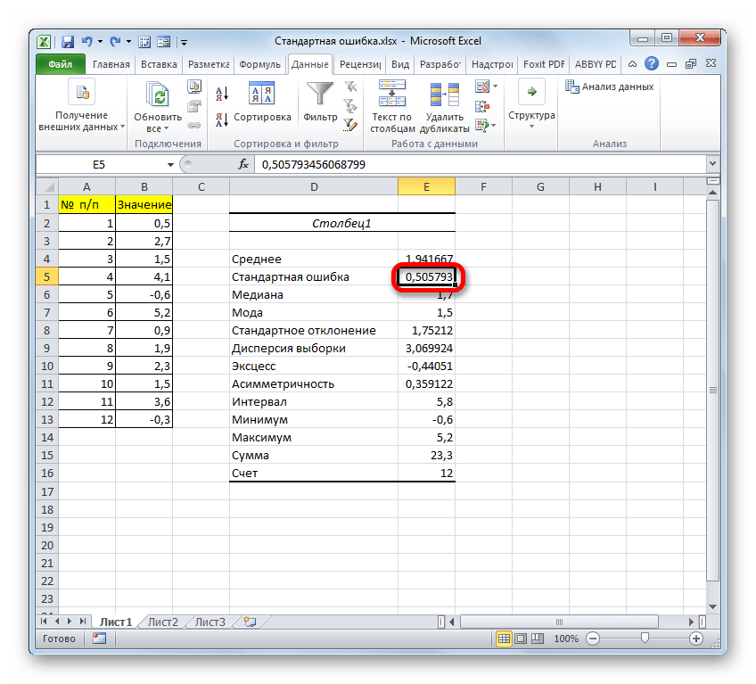
- После этого инструмент «Описательная статистика» выводит результаты обработки выборки на текущий лист. Как видим, это довольно много разноплановых статистических показателей, но среди них есть и нужный нам – «Стандартная ошибка». Он равен числу 0,505793. Это в точности тот же результат, который мы достигли путем применения сложной формулы при описании предыдущего способа.


Урок: Описательная статистика в Экселе
Как видим, в Экселе можно произвести расчет стандартной ошибки двумя способами: применив набор функций и воспользовавшись инструментом пакета анализа «Описательная статистика». Итоговый результат будет абсолютно одинаковый. Поэтому выбор метода зависит от удобства пользователя и поставленной конкретной задачи. Например, если ошибка средней арифметической является только одним из многих статистических показателей выборки, которые нужно рассчитать, то удобнее воспользоваться инструментом «Описательная статистика». Но если вам нужно вычислить исключительно этот показатель, то во избежание нагромождения лишних данных лучше прибегнуть к сложной формуле. В этом случае результат расчета уместится в одной ячейке листа.
Стандартное отклонение и стандартная ошибка: в чем разница?

17 авг. 2022 г.
читать 2 мин
В статистике студенты часто путают два термина: стандартное отклонение и стандартная ошибка .
Стандартное отклонение измеряет, насколько разбросаны значения в наборе данных.
Стандартная ошибка — это стандартное отклонение среднего значения в повторных выборках из совокупности.
Давайте рассмотрим пример, чтобы ясно проиллюстрировать эту идею.
Пример: стандартное отклонение против стандартной ошибки
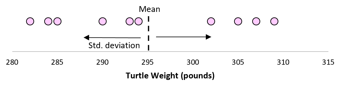
Предположим, мы измеряем вес 10 разных черепах.
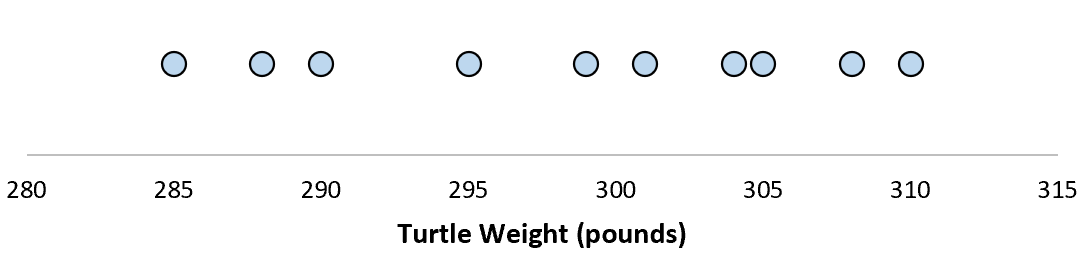
Для этой выборки из 10 черепах мы можем вычислить среднее значение выборки и стандартное отклонение выборки:
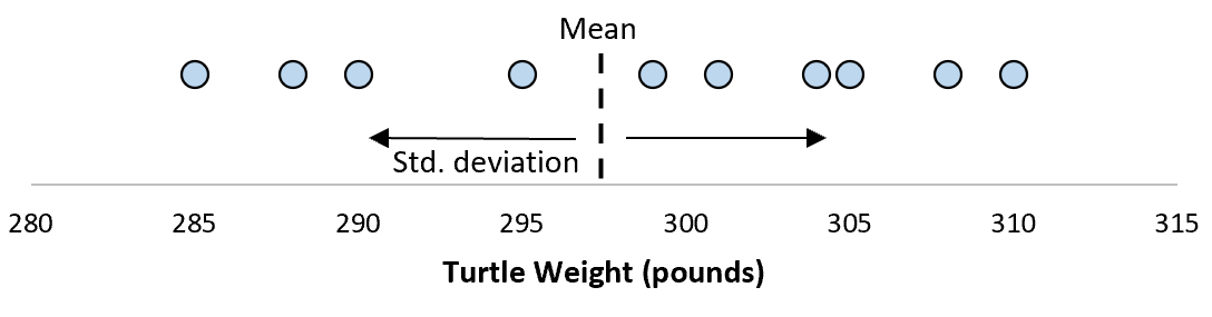
Предположим, что стандартное отклонение оказалось равным 8,68. Это дает нам представление о том, насколько распределен вес этих черепах.
Но предположим, что мы собираем еще одну простую случайную выборку из 10 черепах и также проводим их измерения. Более чем вероятно, что эта выборка из 10 черепах будет иметь немного другое среднее значение и стандартное отклонение, даже если они взяты из одной и той же популяции:
Теперь, если мы представим, что мы берем повторные выборки из одной и той же совокупности и записываем выборочное среднее и выборочное стандартное отклонение для каждой выборки:
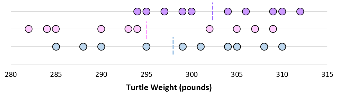
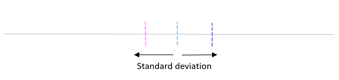
Теперь представьте, что мы наносим каждое среднее значение выборки на одну и ту же строку:

Стандартное отклонение этих средних значений известно как стандартная ошибка.
Формула для фактического расчета стандартной ошибки:
Стандартная ошибка = s/ √n
куда:
- s: стандартное отклонение выборки
- n: размер выборки
Какой смысл использовать стандартную ошибку?
Когда мы вычисляем среднее значение данной выборки, нас на самом деле интересует не среднее значение этой конкретной выборки, а скорее среднее значение большей совокупности, из которой взята выборка.
Однако мы используем выборки, потому что для них гораздо проще собирать данные, чем для всего населения. И, конечно же, среднее значение выборки будет варьироваться от выборки к выборке, поэтому мы используем стандартную ошибку среднего значения как способ измерить, насколько точна наша оценка среднего значения.
Вы заметите из формулы для расчета стандартной ошибки, что по мере увеличения размера выборки (n) стандартная ошибка уменьшается:
Стандартная ошибка = s/ √n
Это должно иметь смысл, поскольку большие размеры выборки уменьшают изменчивость и увеличивают вероятность того, что среднее значение нашей выборки ближе к фактическому среднему значению генеральной совокупности.
Когда использовать стандартное отклонение против стандартной ошибки
Если мы просто заинтересованы в измерении того, насколько разбросаны значения в наборе данных, мы можем использовать стандартное отклонение .
Однако, если мы заинтересованы в количественной оценке неопределенности оценки среднего значения, мы можем использовать стандартную ошибку среднего значения .
В зависимости от вашего конкретного сценария и того, чего вы пытаетесь достичь, вы можете использовать либо стандартное отклонение, либо стандартную ошибку.

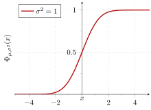
Cumulative probability of a normal distribution with expected value 0 and standard deviation 1
In statistics, the standard deviation is a measure of the amount of variation or dispersion of a set of values.[1] A low standard deviation indicates that the values tend to be close to the mean (also called the expected value) of the set, while a high standard deviation indicates that the values are spread out over a wider range.
Standard deviation may be abbreviated SD, and is most commonly represented in mathematical texts and equations by the lower case Greek letter σ (sigma), for the population standard deviation, or the Latin letter s, for the sample standard deviation.
The standard deviation of a random variable, sample, statistical population, data set, or probability distribution is the square root of its variance. It is algebraically simpler, though in practice less robust, than the average absolute deviation.[2][3] A useful property of the standard deviation is that, unlike the variance, it is expressed in the same unit as the data.
The standard deviation of a population or sample and the standard error of a statistic (e.g., of the sample mean) are quite different, but related. The sample mean’s standard error is the standard deviation of the set of means that would be found by drawing an infinite number of repeated samples from the population and computing a mean for each sample. The mean’s standard error turns out to equal the population standard deviation divided by the square root of the sample size, and is estimated by using the sample standard deviation divided by the square root of the sample size. For example, a poll’s standard error (what is reported as the margin of error of the poll), is the expected standard deviation of the estimated mean if the same poll were to be conducted multiple times. Thus, the standard error estimates the standard deviation of an estimate, which itself measures how much the estimate depends on the particular sample that was taken from the population.
In science, it is common to report both the standard deviation of the data (as a summary statistic) and the standard error of the estimate (as a measure of potential error in the findings). By convention, only effects more than two standard errors away from a null expectation are considered «statistically significant», a safeguard against spurious conclusion that is really due to random sampling error.
When only a sample of data from a population is available, the term standard deviation of the sample or sample standard deviation can refer to either the above-mentioned quantity as applied to those data, or to a modified quantity that is an unbiased estimate of the population standard deviation (the standard deviation of the entire population).
Basic examples[edit]
Population standard deviation of grades of eight students[edit]
Suppose that the entire population of interest is eight students in a particular class. For a finite set of numbers, the population standard deviation is found by taking the square root of the average of the squared deviations of the values subtracted from their average value. The marks of a class of eight students (that is, a statistical population) are the following eight values:

These eight data points have the mean (average) of 5:

First, calculate the deviations of each data point from the mean, and square the result of each:
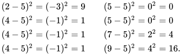
The variance is the mean of these values:

and the population standard deviation is equal to the square root of the variance:

This formula is valid only if the eight values with which we began form the complete population. If the values instead were a random sample drawn from some large parent population (for example, they were 8 students randomly and independently chosen from a class of 2 million), then one divides by 7 (which is n − 1) instead of 8 (which is n) in the denominator of the last formula, and the result is 

Standard deviation of average height for adult men[edit]
If the population of interest is approximately normally distributed, the standard deviation provides information on the proportion of observations above or below certain values. For example, the average height for adult men in the United States is about 70 inches, with a standard deviation of around 3 inches. This means that most men (about 68%, assuming a normal distribution) have a height within 3 inches of the mean (67–73 inches) – one standard deviation – and almost all men (about 95%) have a height within 6 inches of the mean (64–76 inches) – two standard deviations. If the standard deviation were zero, then all men would be exactly 70 inches tall. If the standard deviation were 20 inches, then men would have much more variable heights, with a typical range of about 50–90 inches. Three standard deviations account for 99.73% of the sample population being studied, assuming the distribution is normal or bell-shaped (see the 68–95–99.7 rule, or the empirical rule, for more information).
Definition of population values[edit]
Let μ be the expected value (the average) of random variable X with density f(x):
![{displaystyle mu equiv operatorname {E} [X]=int _{-infty }^{+infty }xf(x),mathrm {d} x}](https://wikimedia.org/api/rest_v1/media/math/render/svg/fb2a61843da0d05619c0dd691dbf3fe315b395ad)
The standard deviation σ of X is defined as
![{displaystyle sigma equiv {sqrt {operatorname {E} left[(X-mu )^{2}right]}}={sqrt {int _{-infty }^{+infty }(x-mu )^{2}f(x),mathrm {d} x}},}](https://wikimedia.org/api/rest_v1/media/math/render/svg/e3a1cfef8ad100fbcae387d9581763f0b389bbc3)
which can be shown to equal
![{textstyle {sqrt {operatorname {E} left[X^{2}right]-(operatorname {E} [X])^{2}}}.}](https://wikimedia.org/api/rest_v1/media/math/render/svg/e2dd8d466c3ecb05713377fefcb7e7f787b29ce7)
Using words, the standard deviation is the square root of the variance of X.
The standard deviation of a probability distribution is the same as that of a random variable having that distribution.
Not all random variables have a standard deviation. If the distribution has fat tails going out to infinity, the standard deviation might not exist, because the integral might not converge. The normal distribution has tails going out to infinity, but its mean and standard deviation do exist, because the tails diminish quickly enough. The Pareto distribution with parameter ![{displaystyle alpha in (1,2]}](https://wikimedia.org/api/rest_v1/media/math/render/svg/782b1d598278b0238ee817c658744e8a7ed3a06e)
Discrete random variable[edit]
In the case where X takes random values from a finite data set x1, x2, …, xN, with each value having the same probability, the standard deviation is
![{displaystyle sigma ={sqrt {{frac {1}{N}}left[(x_{1}-mu )^{2}+(x_{2}-mu )^{2}+cdots +(x_{N}-mu )^{2}right]}},{text{ where }}mu ={frac {1}{N}}(x_{1}+cdots +x_{N}),}](https://wikimedia.org/api/rest_v1/media/math/render/svg/827beb1be760eed3cb07b20d29f01d326f728071)
or, by using summation notation,

If, instead of having equal probabilities, the values have different probabilities, let x1 have probability p1, x2 have probability p2, …, xN have probability pN. In this case, the standard deviation will be

Continuous random variable[edit]
The standard deviation of a continuous real-valued random variable X with probability density function p(x) is

and where the integrals are definite integrals taken for x ranging over the set of possible values of the random variable X.
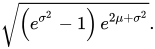
In the case of a parametric family of distributions, the standard deviation can be expressed in terms of the parameters. For example, in the case of the log-normal distribution with parameters μ and σ2, the standard deviation is
Estimation[edit]
One can find the standard deviation of an entire population in cases (such as standardized testing) where every member of a population is sampled. In cases where that cannot be done, the standard deviation σ is estimated by examining a random sample taken from the population and computing a statistic of the sample, which is used as an estimate of the population standard deviation. Such a statistic is called an estimator, and the estimator (or the value of the estimator, namely the estimate) is called a sample standard deviation, and is denoted by s (possibly with modifiers).
Unlike in the case of estimating the population mean, for which the sample mean is a simple estimator with many desirable properties (unbiased, efficient, maximum likelihood), there is no single estimator for the standard deviation with all these properties, and unbiased estimation of standard deviation is a very technically involved problem. Most often, the standard deviation is estimated using the corrected sample standard deviation (using N − 1), defined below, and this is often referred to as the «sample standard deviation», without qualifiers. However, other estimators are better in other respects: the uncorrected estimator (using N) yields lower mean squared error, while using N − 1.5 (for the normal distribution) almost completely eliminates bias.
Uncorrected sample standard deviation[edit]
The formula for the population standard deviation (of a finite population) can be applied to the sample, using the size of the sample as the size of the population (though the actual population size from which the sample is drawn may be much larger). This estimator, denoted by sN, is known as the uncorrected sample standard deviation, or sometimes the standard deviation of the sample (considered as the entire population), and is defined as follows:[6]
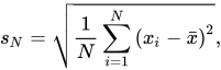
where 

This is a consistent estimator (it converges in probability to the population value as the number of samples goes to infinity), and is the maximum-likelihood estimate when the population is normally distributed.[7] However, this is a biased estimator, as the estimates are generally too low. The bias decreases as sample size grows, dropping off as 1/N, and thus is most significant for small or moderate sample sizes; for 
Corrected sample standard deviation[edit]
If the biased sample variance (the second central moment of the sample, which is a downward-biased estimate of the population variance) is used to compute an estimate of the population’s standard deviation, the result is
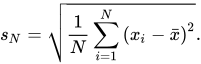
Here taking the square root introduces further downward bias, by Jensen’s inequality, due to the square root’s being a concave function. The bias in the variance is easily corrected, but the bias from the square root is more difficult to correct, and depends on the distribution in question.
An unbiased estimator for the variance is given by applying Bessel’s correction, using N − 1 instead of N to yield the unbiased sample variance, denoted s2:
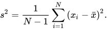
This estimator is unbiased if the variance exists and the sample values are drawn independently with replacement. N − 1 corresponds to the number of degrees of freedom in the vector of deviations from the mean, 
Taking square roots reintroduces bias (because the square root is a nonlinear function which does not commute with the expectation, i.e. often ![{displaystyle E[{sqrt {X}}]neq {sqrt {E[X]}}}](https://wikimedia.org/api/rest_v1/media/math/render/svg/79fa5d2ba8891a41598ddeadc10ba844a20cdfa0)
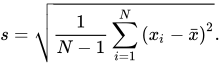
As explained above, while s2 is an unbiased estimator for the population variance, s is still a biased estimator for the population standard deviation, though markedly less biased than the uncorrected sample standard deviation. This estimator is commonly used and generally known simply as the «sample standard deviation». The bias may still be large for small samples (N less than 10). As sample size increases, the amount of bias decreases. We obtain more information and the difference between 

Unbiased sample standard deviation[edit]
For unbiased estimation of standard deviation, there is no formula that works across all distributions, unlike for mean and variance. Instead, s is used as a basis, and is scaled by a correction factor to produce an unbiased estimate. For the normal distribution, an unbiased estimator is given by s/c4, where the correction factor (which depends on N) is given in terms of the Gamma function, and equals:
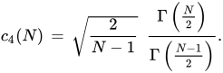
This arises because the sampling distribution of the sample standard deviation follows a (scaled) chi distribution, and the correction factor is the mean of the chi distribution.
An approximation can be given by replacing N − 1 with N − 1.5, yielding:
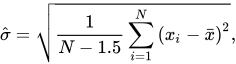
The error in this approximation decays quadratically (as 1/N2), and it is suited for all but the smallest samples or highest precision: for N = 3 the bias is equal to 1.3%, and for N = 9 the bias is already less than 0.1%.
A more accurate approximation is to replace 

For other distributions, the correct formula depends on the distribution, but a rule of thumb is to use the further refinement of the approximation:
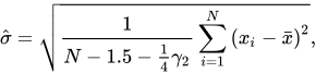
where γ2 denotes the population excess kurtosis. The excess kurtosis may be either known beforehand for certain distributions, or estimated from the data.[9]
Confidence interval of a sampled standard deviation[edit]
The standard deviation we obtain by sampling a distribution is itself not absolutely accurate, both for mathematical reasons (explained here by the confidence interval) and for practical reasons of measurement (measurement error). The mathematical effect can be described by the confidence interval or CI.
To show how a larger sample will make the confidence interval narrower, consider the following examples:
A small population of N = 2 has only 1 degree of freedom for estimating the standard deviation. The result is that a 95% CI of the SD runs from 0.45 × SD to 31.9 × SD; the factors here are as follows:

where 

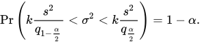
With k = 1, 

A larger population of N = 10 has 9 degrees of freedom for estimating the standard deviation. The same computations as above give us in this case a 95% CI running from 0.69 × SD to 1.83 × SD. So even with a sample population of 10, the actual SD can still be almost a factor 2 higher than the sampled SD. For a sample population N=100, this is down to 0.88 × SD to 1.16 × SD. To be more certain that the sampled SD is close to the actual SD we need to sample a large number of points.
These same formulae can be used to obtain confidence intervals on the variance of residuals from a least squares fit under standard normal theory, where k is now the number of degrees of freedom for error.
Bounds on standard deviation[edit]
For a set of N > 4 data spanning a range of values R, an upper bound on the standard deviation s is given by s = 0.6R.[10]
An estimate of the standard deviation for N > 100 data taken to be approximately normal follows from the heuristic that 95% of the area under the normal curve lies roughly two standard deviations to either side of the mean, so that, with 95% probability the total range of values R represents four standard deviations so that s ≈ R/4. This so-called range rule is useful in sample size estimation, as the range of possible values is easier to estimate than the standard deviation. Other divisors K(N) of the range such that s ≈ R/K(N) are available for other values of N and for non-normal distributions.[11]
Identities and mathematical properties[edit]
The standard deviation is invariant under changes in location, and scales directly with the scale of the random variable. Thus, for a constant c and random variables X and Y:
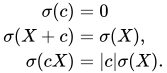
The standard deviation of the sum of two random variables can be related to their individual standard deviations and the covariance between them:

where 

The calculation of the sum of squared deviations can be related to moments calculated directly from the data. In the following formula, the letter E is interpreted to mean expected value, i.e., mean.
![{displaystyle sigma (X)={sqrt {operatorname {E} left[(X-operatorname {E} [X])^{2}right]}}={sqrt {operatorname {E} left[X^{2}right]-(operatorname {E} [X])^{2}}}.}](https://wikimedia.org/api/rest_v1/media/math/render/svg/d3ab12089bd2027790ef060ff7cc2ec05ae2021f)
The sample standard deviation can be computed as:
![{displaystyle s(X)={sqrt {frac {N}{N-1}}}{sqrt {operatorname {E} left[(X-operatorname {E} [X])^{2}right]}}.}](https://wikimedia.org/api/rest_v1/media/math/render/svg/702e9da21c721697e6e81932bf8b7443028f7d6d)
For a finite population with equal probabilities at all points, we have

which means that the standard deviation is equal to the square root of the difference between the average of the squares of the values and the square of the average value.
See computational formula for the variance for proof, and for an analogous result for the sample standard deviation.
Interpretation and application[edit]

Example of samples from two populations with the same mean but different standard deviations. Red population has mean 100 and SD 10; blue population has mean 100 and SD 50.
A large standard deviation indicates that the data points can spread far from the mean and a small standard deviation indicates that they are clustered closely around the mean.
For example, each of the three populations {0, 0, 14, 14}, {0, 6, 8, 14} and {6, 6, 8, 8} has a mean of 7. Their standard deviations are 7, 5, and 1, respectively. The third population has a much smaller standard deviation than the other two because its values are all close to 7. These standard deviations have the same units as the data points themselves. If, for instance, the data set {0, 6, 8, 14} represents the ages of a population of four siblings in years, the standard deviation is 5 years. As another example, the population {1000, 1006, 1008, 1014} may represent the distances traveled by four athletes, measured in meters. It has a mean of 1007 meters, and a standard deviation of 5 meters.
Standard deviation may serve as a measure of uncertainty. In physical science, for example, the reported standard deviation of a group of repeated measurements gives the precision of those measurements. When deciding whether measurements agree with a theoretical prediction, the standard deviation of those measurements is of crucial importance: if the mean of the measurements is too far away from the prediction (with the distance measured in standard deviations), then the theory being tested probably needs to be revised. This makes sense since they fall outside the range of values that could reasonably be expected to occur, if the prediction were correct and the standard deviation appropriately quantified. See prediction interval.
While the standard deviation does measure how far typical values tend to be from the mean, other measures are available. An example is the mean absolute deviation, which might be considered a more direct measure of average distance, compared to the root mean square distance inherent in the standard deviation.
Application examples[edit]
The practical value of understanding the standard deviation of a set of values is in appreciating how much variation there is from the average (mean).
Experiment, industrial and hypothesis testing[edit]
Standard deviation is often used to compare real-world data against a model to test the model.
For example, in industrial applications the weight of products coming off a production line may need to comply with a legally required value. By weighing some fraction of the products an average weight can be found, which will always be slightly different from the long-term average. By using standard deviations, a minimum and maximum value can be calculated that the averaged weight will be within some very high percentage of the time (99.9% or more). If it falls outside the range then the production process may need to be corrected. Statistical tests such as these are particularly important when the testing is relatively expensive. For example, if the product needs to be opened and drained and weighed, or if the product was otherwise used up by the test.
In experimental science, a theoretical model of reality is used. Particle physics conventionally uses a standard of «5 sigma» for the declaration of a discovery. A five-sigma level translates to one chance in 3.5 million that a random fluctuation would yield the result. This level of certainty was required in order to assert that a particle consistent with the Higgs boson had been discovered in two independent experiments at CERN,[12] also leading to the declaration of the first observation of gravitational waves.[13]
Weather[edit]
As a simple example, consider the average daily maximum temperatures for two cities, one inland and one on the coast. It is helpful to understand that the range of daily maximum temperatures for cities near the coast is smaller than for cities inland. Thus, while these two cities may each have the same average maximum temperature, the standard deviation of the daily maximum temperature for the coastal city will be less than that of the inland city as, on any particular day, the actual maximum temperature is more likely to be farther from the average maximum temperature for the inland city than for the coastal one.
Finance[edit]
In finance, standard deviation is often used as a measure of the risk associated with price-fluctuations of a given asset (stocks, bonds, property, etc.), or the risk of a portfolio of assets[14] (actively managed mutual funds, index mutual funds, or ETFs). Risk is an important factor in determining how to efficiently manage a portfolio of investments because it determines the variation in returns on the asset and/or portfolio and gives investors a mathematical basis for investment decisions (known as mean-variance optimization). The fundamental concept of risk is that as it increases, the expected return on an investment should increase as well, an increase known as the risk premium. In other words, investors should expect a higher return on an investment when that investment carries a higher level of risk or uncertainty. When evaluating investments, investors should estimate both the expected return and the uncertainty of future returns. Standard deviation provides a quantified estimate of the uncertainty of future returns.
For example, assume an investor had to choose between two stocks. Stock A over the past 20 years had an average return of 10 percent, with a standard deviation of 20 percentage points (pp) and Stock B, over the same period, had average returns of 12 percent but a higher standard deviation of 30 pp. On the basis of risk and return, an investor may decide that Stock A is the safer choice, because Stock B’s additional two percentage points of return is not worth the additional 10 pp standard deviation (greater risk or uncertainty of the expected return). Stock B is likely to fall short of the initial investment (but also to exceed the initial investment) more often than Stock A under the same circumstances, and is estimated to return only two percent more on average. In this example, Stock A is expected to earn about 10 percent, plus or minus 20 pp (a range of 30 percent to −10 percent), about two-thirds of the future year returns. When considering more extreme possible returns or outcomes in future, an investor should expect results of as much as 10 percent plus or minus 60 pp, or a range from 70 percent to −50 percent, which includes outcomes for three standard deviations from the average return (about 99.7 percent of probable returns).
Calculating the average (or arithmetic mean) of the return of a security over a given period will generate the expected return of the asset. For each period, subtracting the expected return from the actual return results in the difference from the mean. Squaring the difference in each period and taking the average gives the overall variance of the return of the asset. The larger the variance, the greater risk the security carries. Finding the square root of this variance will give the standard deviation of the investment tool in question.
Population standard deviation is used to set the width of Bollinger Bands, a technical analysis tool. For example, the upper Bollinger Band is given as 
Financial time series are known to be non-stationary series, whereas the statistical calculations above, such as standard deviation, apply only to stationary series. To apply the above statistical tools to non-stationary series, the series first must be transformed to a stationary series, enabling use of statistical tools that now have a valid basis from which to work.
Geometric interpretation[edit]
To gain some geometric insights and clarification, we will start with a population of three values, x1, x2, x3. This defines a point P = (x1, x2, x3) in R3. Consider the line L = {(r, r, r) : r ∈ R}. This is the «main diagonal» going through the origin. If our three given values were all equal, then the standard deviation would be zero and P would lie on L. So it is not unreasonable to assume that the standard deviation is related to the distance of P to L. That is indeed the case. To move orthogonally from L to the point P, one begins at the point:
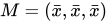
whose coordinates are the mean of the values we started out with.
A little algebra shows that the distance between P and M (which is the same as the orthogonal distance between P and the line L) 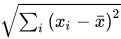
Chebyshev’s inequality[edit]
An observation is rarely more than a few standard deviations away from the mean. Chebyshev’s inequality ensures that, for all distributions for which the standard deviation is defined, the amount of data within a number of standard deviations of the mean is at least as much as given in the following table.
| Distance from mean | Minimum population |
|---|---|
 |
50% |
| 2σ | 75% |
| 3σ | 89% |
| 4σ | 94% |
| 5σ | 96% |
| 6σ | 97% |
 |
 [15] [15]
|
 |

|
Rules for normally distributed data[edit]
Dark blue is one standard deviation on either side of the mean. For the normal distribution, this accounts for 68.27 percent of the set; while two standard deviations from the mean (medium and dark blue) account for 95.45 percent; three standard deviations (light, medium, and dark blue) account for 99.73 percent; and four standard deviations account for 99.994 percent. The two points of the curve that are one standard deviation from the mean are also the inflection points.
The central limit theorem states that the distribution of an average of many independent, identically distributed random variables tends toward the famous bell-shaped normal distribution with a probability density function of
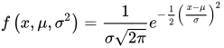
where μ is the expected value of the random variables, σ equals their distribution’s standard deviation divided by n1/2, and n is the number of random variables. The standard deviation therefore is simply a scaling variable that adjusts how broad the curve will be, though it also appears in the normalizing constant.
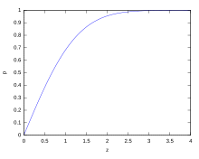
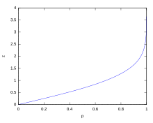
If a data distribution is approximately normal, then the proportion of data values within z standard deviations of the mean is defined by:
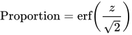
where 
.[16]
If a data distribution is approximately normal then about 68 percent of the data values are within one standard deviation of the mean (mathematically, μ ± σ, where μ is the arithmetic mean), about 95 percent are within two standard deviations (μ ± 2σ), and about 99.7 percent lie within three standard deviations (μ ± 3σ). This is known as the 68–95–99.7 rule, or the empirical rule.
For various values of z, the percentage of values expected to lie in and outside the symmetric interval, CI = (−zσ, zσ), are as follows:
| Confidence interval |
Proportion within | Proportion without | |
|---|---|---|---|
| Percentage | Percentage | Fraction | |
| 0.318639σ | 25% | 75% | 3 / 4 |
| 0.674490σ | 50% | 50% | 1 / 2 |
| 0.977925σ | 66.6667% | 33.3333% | 1 / 3 |
| 0.994458σ | 68% | 32% | 1 / 3.125 |
| 1σ | 68.2689492% | 31.7310508% | 1 / 3.1514872 |
| 1.281552σ | 80% | 20% | 1 / 5 |
| 1.644854σ | 90% | 10% | 1 / 10 |
| 1.959964σ | 95% | 5% | 1 / 20 |
| 2σ | 95.4499736% | 4.5500264% | 1 / 21.977895 |
| 2.575829σ | 99% | 1% | 1 / 100 |
| 3σ | 99.7300204% | 0.2699796% | 1 / 370.398 |
| 3.290527σ | 99.9% | 0.1% | 1 / 1000 |
| 3.890592σ | 99.99% | 0.01% | 1 / 10000 |
| 4σ | 99.993666% | 0.006334% | 1 / 15787 |
| 4.417173σ | 99.999% | 0.001% | 1 / 100000 |
| 4.5σ | 99.9993204653751% | 0.0006795346249% | 1 / 147159.5358 6.8 / 1000000 |
| 4.891638σ | 99.9999% | 0.0001% | 1 / 1000000 |
| 5σ | 99.9999426697% | 0.0000573303% | 1 / 1744278 |
| 5.326724σ | 99.99999% | 0.00001% | 1 / 10000000 |
| 5.730729σ | 99.999999% | 0.000001% | 1 / 100000000 |
| 6σ | 99.9999998027% | 0.0000001973% | 1 / 506797346 |
| 6.109410σ | 99.9999999% | 0.0000001% | 1 / 1000000000 |
| 6.466951σ | 99.99999999% | 0.00000001% | 1 / 10000000000 |
| 6.806502σ | 99.999999999% | 0.000000001% | 1 / 100000000000 |
| 7σ | 99.9999999997440% | 0.000000000256% | 1 / 390682215445 |
Relationship between standard deviation and mean[edit]
The mean and the standard deviation of a set of data are descriptive statistics usually reported together. In a certain sense, the standard deviation is a «natural» measure of statistical dispersion if the center of the data is measured about the mean. This is because the standard deviation from the mean is smaller than from any other point. The precise statement is the following: suppose x1, …, xn are real numbers and define the function:
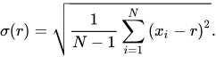
Using calculus or by completing the square, it is possible to show that σ(r) has a unique minimum at the mean:

Variability can also be measured by the coefficient of variation, which is the ratio of the standard deviation to the mean. It is a dimensionless number.
Standard deviation of the mean[edit]
Often, we want some information about the precision of the mean we obtained. We can obtain this by determining the standard deviation of the sampled mean. Assuming statistical independence of the values in the sample, the standard deviation of the mean is related to the standard deviation of the distribution by:
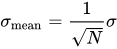
where N is the number of observations in the sample used to estimate the mean. This can easily be proven with (see basic properties of the variance):

(Statistical independence is assumed.)

hence
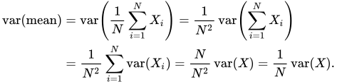
Resulting in:
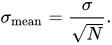
In order to estimate the standard deviation of the mean 

Rapid calculation methods[edit]
The following two formulas can represent a running (repeatedly updated) standard deviation. A set of two power sums s1 and s2 are computed over a set of N values of x, denoted as x1, …, xN:

Given the results of these running summations, the values N, s1, s2 can be used at any time to compute the current value of the running standard deviation:
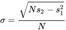
Where N, as mentioned above, is the size of the set of values (or can also be regarded as s0).
Similarly for sample standard deviation,
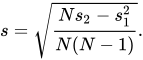
In a computer implementation, as the two sj sums become large, we need to consider round-off error, arithmetic overflow, and arithmetic underflow. The method below calculates the running sums method with reduced rounding errors.[17] This is a «one pass» algorithm for calculating variance of n samples without the need to store prior data during the calculation. Applying this method to a time series will result in successive values of standard deviation corresponding to n data points as n grows larger with each new sample, rather than a constant-width sliding window calculation.
For k = 1, …, n:
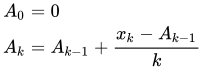
where A is the mean value.

Note: 


Sample variance:

Population variance:

Weighted calculation[edit]
When the values xi are weighted with unequal weights wi, the power sums s0, s1, s2 are each computed as:
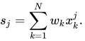
And the standard deviation equations remain unchanged. s0 is now the sum of the weights and not the number of samples N.
The incremental method with reduced rounding errors can also be applied, with some additional complexity.
A running sum of weights must be computed for each k from 1 to n:
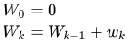
and places where 1/n is used above must be replaced by wi/Wn:
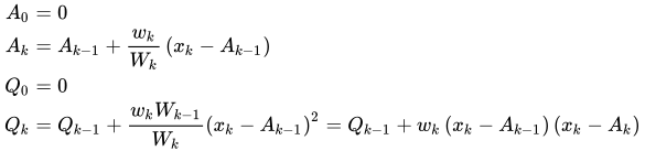
In the final division,

and
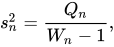
or

where n is the total number of elements, and n’ is the number of elements with non-zero weights.
The above formulas become equal to the simpler formulas given above if weights are taken as equal to one.
History[edit]
The term standard deviation was first used in writing by Karl Pearson in 1894, following his use of it in lectures.[18][19] This was as a replacement for earlier alternative names for the same idea: for example, Gauss used mean error.[20]
Higher dimensions[edit]
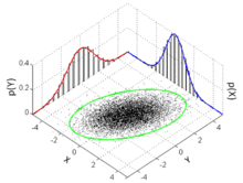
The standard deviation ellipse (green) of a two-dimensional normal distribution
In two dimensions, the standard deviation can be illustrated with the standard deviation ellipse (see Multivariate normal distribution § Geometric interpretation).
See also[edit]
- 68–95–99.7 rule
- Accuracy and precision
- Chebyshev’s inequality An inequality on location and scale parameters
- Coefficient of variation
- Cumulant
- Deviation (statistics)
- Distance correlation Distance standard deviation
- Error bar
- Geometric standard deviation
- Mahalanobis distance generalizing number of standard deviations to the mean
- Mean absolute error
- Pooled variance
- Propagation of uncertainty
- Percentile
- Raw data
- Robust standard deviation
- Root mean square
- Sample size
- Samuelson’s inequality
- Six Sigma
- Standard error
- Standard score
- Yamartino method for calculating standard deviation of wind direction
References[edit]
- ^ Bland, J.M.; Altman, D.G. (1996). «Statistics notes: measurement error». BMJ. 312 (7047): 1654. doi:10.1136/bmj.312.7047.1654. PMC 2351401. PMID 8664723.
- ^ Gauss, Carl Friedrich (1816). «Bestimmung der Genauigkeit der Beobachtungen». Zeitschrift für Astronomie und Verwandte Wissenschaften. 1: 187–197.
- ^ Walker, Helen (1931). Studies in the History of the Statistical Method. Baltimore, MD: Williams & Wilkins Co. pp. 24–25.
- ^ Weisstein, Eric W. «Bessel’s Correction». MathWorld.
- ^ «Standard Deviation Formulas». www.mathsisfun.com. Retrieved 21 August 2020.
- ^ Weisstein, Eric W. «Standard Deviation». mathworld.wolfram.com. Retrieved 21 August 2020.
- ^ «Consistent estimator». www.statlect.com. Retrieved 10 October 2022.
- ^ Gurland, John; Tripathi, Ram C. (1971), «A Simple Approximation for Unbiased Estimation of the Standard Deviation», The American Statistician, 25 (4): 30–32, doi:10.2307/2682923, JSTOR 2682923
- ^ «Standard Deviation Calculator». PureCalculators. 11 July 2021. Retrieved 14 September 2021.
- ^ Shiffler, Ronald E.; Harsha, Phillip D. (1980). «Upper and Lower Bounds for the Sample Standard Deviation». Teaching Statistics. 2 (3): 84–86. doi:10.1111/j.1467-9639.1980.tb00398.x.
- ^ Browne, Richard H. (2001). «Using the Sample Range as a Basis for Calculating Sample Size in Power Calculations». The American Statistician. 55 (4): 293–298. doi:10.1198/000313001753272420. JSTOR 2685690. S2CID 122328846.
- ^ «CERN experiments observe particle consistent with long-sought Higgs boson | CERN press office». Press.web.cern.ch. 4 July 2012. Archived from the original on 25 March 2016. Retrieved 30 May 2015.
- ^ LIGO Scientific Collaboration, Virgo Collaboration (2016), «Observation of Gravitational Waves from a Binary Black Hole Merger», Physical Review Letters, 116 (6): 061102, arXiv:1602.03837, Bibcode:2016PhRvL.116f1102A, doi:10.1103/PhysRevLett.116.061102, PMID 26918975, S2CID 124959784
- ^ «What is Standard Deviation». Pristine. Retrieved 29 October 2011.
- ^ Ghahramani, Saeed (2000). Fundamentals of Probability (2nd ed.). New Jersey: Prentice Hall. p. 438. ISBN 9780130113290.
- ^ Eric W. Weisstein. «Distribution Function». MathWorld—A Wolfram Web Resource. Retrieved 30 September 2014.
- ^ Welford, BP (August 1962). «Note on a Method for Calculating Corrected Sums of Squares and Products». Technometrics. 4 (3): 419–420. CiteSeerX 10.1.1.302.7503. doi:10.1080/00401706.1962.10490022.
- ^ Dodge, Yadolah (2003). The Oxford Dictionary of Statistical Terms. Oxford University Press. ISBN 978-0-19-920613-1.
- ^ Pearson, Karl (1894). «On the dissection of asymmetrical frequency curves». Philosophical Transactions of the Royal Society A. 185: 71–110. Bibcode:1894RSPTA.185…71P. doi:10.1098/rsta.1894.0003.
- ^ Miller, Jeff. «Earliest Known Uses of Some of the Words of Mathematics».
External links[edit]
- «Quadratic deviation», Encyclopedia of Mathematics, EMS Press, 2001 [1994]
- «Standard Deviation Calculator»
Cumulative probability of a normal distribution with expected value 0 and standard deviation 1
In statistics, the standard deviation is a measure of the amount of variation or dispersion of a set of values.[1] A low standard deviation indicates that the values tend to be close to the mean (also called the expected value) of the set, while a high standard deviation indicates that the values are spread out over a wider range.
Standard deviation may be abbreviated SD, and is most commonly represented in mathematical texts and equations by the lower case Greek letter σ (sigma), for the population standard deviation, or the Latin letter s, for the sample standard deviation.
The standard deviation of a random variable, sample, statistical population, data set, or probability distribution is the square root of its variance. It is algebraically simpler, though in practice less robust, than the average absolute deviation.[2][3] A useful property of the standard deviation is that, unlike the variance, it is expressed in the same unit as the data.
The standard deviation of a population or sample and the standard error of a statistic (e.g., of the sample mean) are quite different, but related. The sample mean’s standard error is the standard deviation of the set of means that would be found by drawing an infinite number of repeated samples from the population and computing a mean for each sample. The mean’s standard error turns out to equal the population standard deviation divided by the square root of the sample size, and is estimated by using the sample standard deviation divided by the square root of the sample size. For example, a poll’s standard error (what is reported as the margin of error of the poll), is the expected standard deviation of the estimated mean if the same poll were to be conducted multiple times. Thus, the standard error estimates the standard deviation of an estimate, which itself measures how much the estimate depends on the particular sample that was taken from the population.
In science, it is common to report both the standard deviation of the data (as a summary statistic) and the standard error of the estimate (as a measure of potential error in the findings). By convention, only effects more than two standard errors away from a null expectation are considered «statistically significant», a safeguard against spurious conclusion that is really due to random sampling error.
When only a sample of data from a population is available, the term standard deviation of the sample or sample standard deviation can refer to either the above-mentioned quantity as applied to those data, or to a modified quantity that is an unbiased estimate of the population standard deviation (the standard deviation of the entire population).
Basic examples[edit]
Population standard deviation of grades of eight students[edit]
Suppose that the entire population of interest is eight students in a particular class. For a finite set of numbers, the population standard deviation is found by taking the square root of the average of the squared deviations of the values subtracted from their average value. The marks of a class of eight students (that is, a statistical population) are the following eight values:
These eight data points have the mean (average) of 5:
First, calculate the deviations of each data point from the mean, and square the result of each:
The variance is the mean of these values:
and the population standard deviation is equal to the square root of the variance:
This formula is valid only if the eight values with which we began form the complete population. If the values instead were a random sample drawn from some large parent population (for example, they were 8 students randomly and independently chosen from a class of 2 million), then one divides by 7 (which is n − 1) instead of 8 (which is n) in the denominator of the last formula, and the result is
Standard deviation of average height for adult men[edit]
If the population of interest is approximately normally distributed, the standard deviation provides information on the proportion of observations above or below certain values. For example, the average height for adult men in the United States is about 70 inches, with a standard deviation of around 3 inches. This means that most men (about 68%, assuming a normal distribution) have a height within 3 inches of the mean (67–73 inches) – one standard deviation – and almost all men (about 95%) have a height within 6 inches of the mean (64–76 inches) – two standard deviations. If the standard deviation were zero, then all men would be exactly 70 inches tall. If the standard deviation were 20 inches, then men would have much more variable heights, with a typical range of about 50–90 inches. Three standard deviations account for 99.73% of the sample population being studied, assuming the distribution is normal or bell-shaped (see the 68–95–99.7 rule, or the empirical rule, for more information).
Definition of population values[edit]
Let μ be the expected value (the average) of random variable X with density f(x):
The standard deviation σ of X is defined as
which can be shown to equal
Using words, the standard deviation is the square root of the variance of X.
The standard deviation of a probability distribution is the same as that of a random variable having that distribution.
Not all random variables have a standard deviation. If the distribution has fat tails going out to infinity, the standard deviation might not exist, because the integral might not converge. The normal distribution has tails going out to infinity, but its mean and standard deviation do exist, because the tails diminish quickly enough. The Pareto distribution with parameter
Discrete random variable[edit]
In the case where X takes random values from a finite data set x1, x2, …, xN, with each value having the same probability, the standard deviation is
or, by using summation notation,
If, instead of having equal probabilities, the values have different probabilities, let x1 have probability p1, x2 have probability p2, …, xN have probability pN. In this case, the standard deviation will be
Continuous random variable[edit]
The standard deviation of a continuous real-valued random variable X with probability density function p(x) is
and where the integrals are definite integrals taken for x ranging over the set of possible values of the random variable X.
In the case of a parametric family of distributions, the standard deviation can be expressed in terms of the parameters. For example, in the case of the log-normal distribution with parameters μ and σ2, the standard deviation is
Estimation[edit]
One can find the standard deviation of an entire population in cases (such as standardized testing) where every member of a population is sampled. In cases where that cannot be done, the standard deviation σ is estimated by examining a random sample taken from the population and computing a statistic of the sample, which is used as an estimate of the population standard deviation. Such a statistic is called an estimator, and the estimator (or the value of the estimator, namely the estimate) is called a sample standard deviation, and is denoted by s (possibly with modifiers).
Unlike in the case of estimating the population mean, for which the sample mean is a simple estimator with many desirable properties (unbiased, efficient, maximum likelihood), there is no single estimator for the standard deviation with all these properties, and unbiased estimation of standard deviation is a very technically involved problem. Most often, the standard deviation is estimated using the corrected sample standard deviation (using N − 1), defined below, and this is often referred to as the «sample standard deviation», without qualifiers. However, other estimators are better in other respects: the uncorrected estimator (using N) yields lower mean squared error, while using N − 1.5 (for the normal distribution) almost completely eliminates bias.
Uncorrected sample standard deviation[edit]
The formula for the population standard deviation (of a finite population) can be applied to the sample, using the size of the sample as the size of the population (though the actual population size from which the sample is drawn may be much larger). This estimator, denoted by sN, is known as the uncorrected sample standard deviation, or sometimes the standard deviation of the sample (considered as the entire population), and is defined as follows:[6]
where
This is a consistent estimator (it converges in probability to the population value as the number of samples goes to infinity), and is the maximum-likelihood estimate when the population is normally distributed.[7] However, this is a biased estimator, as the estimates are generally too low. The bias decreases as sample size grows, dropping off as 1/N, and thus is most significant for small or moderate sample sizes; for
Corrected sample standard deviation[edit]
If the biased sample variance (the second central moment of the sample, which is a downward-biased estimate of the population variance) is used to compute an estimate of the population’s standard deviation, the result is
Here taking the square root introduces further downward bias, by Jensen’s inequality, due to the square root’s being a concave function. The bias in the variance is easily corrected, but the bias from the square root is more difficult to correct, and depends on the distribution in question.
An unbiased estimator for the variance is given by applying Bessel’s correction, using N − 1 instead of N to yield the unbiased sample variance, denoted s2:
This estimator is unbiased if the variance exists and the sample values are drawn independently with replacement. N − 1 corresponds to the number of degrees of freedom in the vector of deviations from the mean,
Taking square roots reintroduces bias (because the square root is a nonlinear function which does not commute with the expectation, i.e. often
As explained above, while s2 is an unbiased estimator for the population variance, s is still a biased estimator for the population standard deviation, though markedly less biased than the uncorrected sample standard deviation. This estimator is commonly used and generally known simply as the «sample standard deviation». The bias may still be large for small samples (N less than 10). As sample size increases, the amount of bias decreases. We obtain more information and the difference between
Unbiased sample standard deviation[edit]
For unbiased estimation of standard deviation, there is no formula that works across all distributions, unlike for mean and variance. Instead, s is used as a basis, and is scaled by a correction factor to produce an unbiased estimate. For the normal distribution, an unbiased estimator is given by s/c4, where the correction factor (which depends on N) is given in terms of the Gamma function, and equals:
This arises because the sampling distribution of the sample standard deviation follows a (scaled) chi distribution, and the correction factor is the mean of the chi distribution.
An approximation can be given by replacing N − 1 with N − 1.5, yielding:
The error in this approximation decays quadratically (as 1/N2), and it is suited for all but the smallest samples or highest precision: for N = 3 the bias is equal to 1.3%, and for N = 9 the bias is already less than 0.1%.
A more accurate approximation is to replace
For other distributions, the correct formula depends on the distribution, but a rule of thumb is to use the further refinement of the approximation:
where γ2 denotes the population excess kurtosis. The excess kurtosis may be either known beforehand for certain distributions, or estimated from the data.[9]
Confidence interval of a sampled standard deviation[edit]
The standard deviation we obtain by sampling a distribution is itself not absolutely accurate, both for mathematical reasons (explained here by the confidence interval) and for practical reasons of measurement (measurement error). The mathematical effect can be described by the confidence interval or CI.
To show how a larger sample will make the confidence interval narrower, consider the following examples:
A small population of N = 2 has only 1 degree of freedom for estimating the standard deviation. The result is that a 95% CI of the SD runs from 0.45 × SD to 31.9 × SD; the factors here are as follows:
where
With k = 1,
A larger population of N = 10 has 9 degrees of freedom for estimating the standard deviation. The same computations as above give us in this case a 95% CI running from 0.69 × SD to 1.83 × SD. So even with a sample population of 10, the actual SD can still be almost a factor 2 higher than the sampled SD. For a sample population N=100, this is down to 0.88 × SD to 1.16 × SD. To be more certain that the sampled SD is close to the actual SD we need to sample a large number of points.
These same formulae can be used to obtain confidence intervals on the variance of residuals from a least squares fit under standard normal theory, where k is now the number of degrees of freedom for error.
Bounds on standard deviation[edit]
For a set of N > 4 data spanning a range of values R, an upper bound on the standard deviation s is given by s = 0.6R.[10]
An estimate of the standard deviation for N > 100 data taken to be approximately normal follows from the heuristic that 95% of the area under the normal curve lies roughly two standard deviations to either side of the mean, so that, with 95% probability the total range of values R represents four standard deviations so that s ≈ R/4. This so-called range rule is useful in sample size estimation, as the range of possible values is easier to estimate than the standard deviation. Other divisors K(N) of the range such that s ≈ R/K(N) are available for other values of N and for non-normal distributions.[11]
Identities and mathematical properties[edit]
The standard deviation is invariant under changes in location, and scales directly with the scale of the random variable. Thus, for a constant c and random variables X and Y:
The standard deviation of the sum of two random variables can be related to their individual standard deviations and the covariance between them:
where
The calculation of the sum of squared deviations can be related to moments calculated directly from the data. In the following formula, the letter E is interpreted to mean expected value, i.e., mean.
The sample standard deviation can be computed as:
For a finite population with equal probabilities at all points, we have
which means that the standard deviation is equal to the square root of the difference between the average of the squares of the values and the square of the average value.
See computational formula for the variance for proof, and for an analogous result for the sample standard deviation.
Interpretation and application[edit]
Example of samples from two populations with the same mean but different standard deviations. Red population has mean 100 and SD 10; blue population has mean 100 and SD 50.
A large standard deviation indicates that the data points can spread far from the mean and a small standard deviation indicates that they are clustered closely around the mean.
For example, each of the three populations {0, 0, 14, 14}, {0, 6, 8, 14} and {6, 6, 8, 8} has a mean of 7. Their standard deviations are 7, 5, and 1, respectively. The third population has a much smaller standard deviation than the other two because its values are all close to 7. These standard deviations have the same units as the data points themselves. If, for instance, the data set {0, 6, 8, 14} represents the ages of a population of four siblings in years, the standard deviation is 5 years. As another example, the population {1000, 1006, 1008, 1014} may represent the distances traveled by four athletes, measured in meters. It has a mean of 1007 meters, and a standard deviation of 5 meters.
Standard deviation may serve as a measure of uncertainty. In physical science, for example, the reported standard deviation of a group of repeated measurements gives the precision of those measurements. When deciding whether measurements agree with a theoretical prediction, the standard deviation of those measurements is of crucial importance: if the mean of the measurements is too far away from the prediction (with the distance measured in standard deviations), then the theory being tested probably needs to be revised. This makes sense since they fall outside the range of values that could reasonably be expected to occur, if the prediction were correct and the standard deviation appropriately quantified. See prediction interval.
While the standard deviation does measure how far typical values tend to be from the mean, other measures are available. An example is the mean absolute deviation, which might be considered a more direct measure of average distance, compared to the root mean square distance inherent in the standard deviation.
Application examples[edit]
The practical value of understanding the standard deviation of a set of values is in appreciating how much variation there is from the average (mean).
Experiment, industrial and hypothesis testing[edit]
Standard deviation is often used to compare real-world data against a model to test the model.
For example, in industrial applications the weight of products coming off a production line may need to comply with a legally required value. By weighing some fraction of the products an average weight can be found, which will always be slightly different from the long-term average. By using standard deviations, a minimum and maximum value can be calculated that the averaged weight will be within some very high percentage of the time (99.9% or more). If it falls outside the range then the production process may need to be corrected. Statistical tests such as these are particularly important when the testing is relatively expensive. For example, if the product needs to be opened and drained and weighed, or if the product was otherwise used up by the test.
In experimental science, a theoretical model of reality is used. Particle physics conventionally uses a standard of «5 sigma» for the declaration of a discovery. A five-sigma level translates to one chance in 3.5 million that a random fluctuation would yield the result. This level of certainty was required in order to assert that a particle consistent with the Higgs boson had been discovered in two independent experiments at CERN,[12] also leading to the declaration of the first observation of gravitational waves.[13]
Weather[edit]
As a simple example, consider the average daily maximum temperatures for two cities, one inland and one on the coast. It is helpful to understand that the range of daily maximum temperatures for cities near the coast is smaller than for cities inland. Thus, while these two cities may each have the same average maximum temperature, the standard deviation of the daily maximum temperature for the coastal city will be less than that of the inland city as, on any particular day, the actual maximum temperature is more likely to be farther from the average maximum temperature for the inland city than for the coastal one.
Finance[edit]
In finance, standard deviation is often used as a measure of the risk associated with price-fluctuations of a given asset (stocks, bonds, property, etc.), or the risk of a portfolio of assets[14] (actively managed mutual funds, index mutual funds, or ETFs). Risk is an important factor in determining how to efficiently manage a portfolio of investments because it determines the variation in returns on the asset and/or portfolio and gives investors a mathematical basis for investment decisions (known as mean-variance optimization). The fundamental concept of risk is that as it increases, the expected return on an investment should increase as well, an increase known as the risk premium. In other words, investors should expect a higher return on an investment when that investment carries a higher level of risk or uncertainty. When evaluating investments, investors should estimate both the expected return and the uncertainty of future returns. Standard deviation provides a quantified estimate of the uncertainty of future returns.
For example, assume an investor had to choose between two stocks. Stock A over the past 20 years had an average return of 10 percent, with a standard deviation of 20 percentage points (pp) and Stock B, over the same period, had average returns of 12 percent but a higher standard deviation of 30 pp. On the basis of risk and return, an investor may decide that Stock A is the safer choice, because Stock B’s additional two percentage points of return is not worth the additional 10 pp standard deviation (greater risk or uncertainty of the expected return). Stock B is likely to fall short of the initial investment (but also to exceed the initial investment) more often than Stock A under the same circumstances, and is estimated to return only two percent more on average. In this example, Stock A is expected to earn about 10 percent, plus or minus 20 pp (a range of 30 percent to −10 percent), about two-thirds of the future year returns. When considering more extreme possible returns or outcomes in future, an investor should expect results of as much as 10 percent plus or minus 60 pp, or a range from 70 percent to −50 percent, which includes outcomes for three standard deviations from the average return (about 99.7 percent of probable returns).
Calculating the average (or arithmetic mean) of the return of a security over a given period will generate the expected return of the asset. For each period, subtracting the expected return from the actual return results in the difference from the mean. Squaring the difference in each period and taking the average gives the overall variance of the return of the asset. The larger the variance, the greater risk the security carries. Finding the square root of this variance will give the standard deviation of the investment tool in question.
Population standard deviation is used to set the width of Bollinger Bands, a technical analysis tool. For example, the upper Bollinger Band is given as
Financial time series are known to be non-stationary series, whereas the statistical calculations above, such as standard deviation, apply only to stationary series. To apply the above statistical tools to non-stationary series, the series first must be transformed to a stationary series, enabling use of statistical tools that now have a valid basis from which to work.
Geometric interpretation[edit]
To gain some geometric insights and clarification, we will start with a population of three values, x1, x2, x3. This defines a point P = (x1, x2, x3) in R3. Consider the line L = {(r, r, r) : r ∈ R}. This is the «main diagonal» going through the origin. If our three given values were all equal, then the standard deviation would be zero and P would lie on L. So it is not unreasonable to assume that the standard deviation is related to the distance of P to L. That is indeed the case. To move orthogonally from L to the point P, one begins at the point:
whose coordinates are the mean of the values we started out with.
A little algebra shows that the distance between P and M (which is the same as the orthogonal distance between P and the line L)
Chebyshev’s inequality[edit]
An observation is rarely more than a few standard deviations away from the mean. Chebyshev’s inequality ensures that, for all distributions for which the standard deviation is defined, the amount of data within a number of standard deviations of the mean is at least as much as given in the following table.
| Distance from mean | Minimum population |
|---|---|
|
50% |
| 2σ | 75% |
| 3σ | 89% |
| 4σ | 94% |
| 5σ | 96% |
| 6σ | 97% |
|
[15]
|
|
|
Rules for normally distributed data[edit]
Dark blue is one standard deviation on either side of the mean. For the normal distribution, this accounts for 68.27 percent of the set; while two standard deviations from the mean (medium and dark blue) account for 95.45 percent; three standard deviations (light, medium, and dark blue) account for 99.73 percent; and four standard deviations account for 99.994 percent. The two points of the curve that are one standard deviation from the mean are also the inflection points.
The central limit theorem states that the distribution of an average of many independent, identically distributed random variables tends toward the famous bell-shaped normal distribution with a probability density function of
where μ is the expected value of the random variables, σ equals their distribution’s standard deviation divided by n1/2, and n is the number of random variables. The standard deviation therefore is simply a scaling variable that adjusts how broad the curve will be, though it also appears in the normalizing constant.
If a data distribution is approximately normal, then the proportion of data values within z standard deviations of the mean is defined by:
where
If a data distribution is approximately normal then about 68 percent of the data values are within one standard deviation of the mean (mathematically, μ ± σ, where μ is the arithmetic mean), about 95 percent are within two standard deviations (μ ± 2σ), and about 99.7 percent lie within three standard deviations (μ ± 3σ). This is known as the 68–95–99.7 rule, or the empirical rule.
For various values of z, the percentage of values expected to lie in and outside the symmetric interval, CI = (−zσ, zσ), are as follows:
| Confidence interval |
Proportion within | Proportion without | |
|---|---|---|---|
| Percentage | Percentage | Fraction | |
| 0.318639σ | 25% | 75% | 3 / 4 |
| 0.674490σ | 50% | 50% | 1 / 2 |
| 0.977925σ | 66.6667% | 33.3333% | 1 / 3 |
| 0.994458σ | 68% | 32% | 1 / 3.125 |
| 1σ | 68.2689492% | 31.7310508% | 1 / 3.1514872 |
| 1.281552σ | 80% | 20% | 1 / 5 |
| 1.644854σ | 90% | 10% | 1 / 10 |
| 1.959964σ | 95% | 5% | 1 / 20 |
| 2σ | 95.4499736% | 4.5500264% | 1 / 21.977895 |
| 2.575829σ | 99% | 1% | 1 / 100 |
| 3σ | 99.7300204% | 0.2699796% | 1 / 370.398 |
| 3.290527σ | 99.9% | 0.1% | 1 / 1000 |
| 3.890592σ | 99.99% | 0.01% | 1 / 10000 |
| 4σ | 99.993666% | 0.006334% | 1 / 15787 |
| 4.417173σ | 99.999% | 0.001% | 1 / 100000 |
| 4.5σ | 99.9993204653751% | 0.0006795346249% | 1 / 147159.5358 6.8 / 1000000 |
| 4.891638σ | 99.9999% | 0.0001% | 1 / 1000000 |
| 5σ | 99.9999426697% | 0.0000573303% | 1 / 1744278 |
| 5.326724σ | 99.99999% | 0.00001% | 1 / 10000000 |
| 5.730729σ | 99.999999% | 0.000001% | 1 / 100000000 |
| 6σ | 99.9999998027% | 0.0000001973% | 1 / 506797346 |
| 6.109410σ | 99.9999999% | 0.0000001% | 1 / 1000000000 |
| 6.466951σ | 99.99999999% | 0.00000001% | 1 / 10000000000 |
| 6.806502σ | 99.999999999% | 0.000000001% | 1 / 100000000000 |
| 7σ | 99.9999999997440% | 0.000000000256% | 1 / 390682215445 |
Relationship between standard deviation and mean[edit]
The mean and the standard deviation of a set of data are descriptive statistics usually reported together. In a certain sense, the standard deviation is a «natural» measure of statistical dispersion if the center of the data is measured about the mean. This is because the standard deviation from the mean is smaller than from any other point. The precise statement is the following: suppose x1, …, xn are real numbers and define the function:
Using calculus or by completing the square, it is possible to show that σ(r) has a unique minimum at the mean:
Variability can also be measured by the coefficient of variation, which is the ratio of the standard deviation to the mean. It is a dimensionless number.
Standard deviation of the mean[edit]
Often, we want some information about the precision of the mean we obtained. We can obtain this by determining the standard deviation of the sampled mean. Assuming statistical independence of the values in the sample, the standard deviation of the mean is related to the standard deviation of the distribution by:
where N is the number of observations in the sample used to estimate the mean. This can easily be proven with (see basic properties of the variance):
(Statistical independence is assumed.)
hence
Resulting in:
In order to estimate the standard deviation of the mean
Rapid calculation methods[edit]
The following two formulas can represent a running (repeatedly updated) standard deviation. A set of two power sums s1 and s2 are computed over a set of N values of x, denoted as x1, …, xN:
Given the results of these running summations, the values N, s1, s2 can be used at any time to compute the current value of the running standard deviation:
Where N, as mentioned above, is the size of the set of values (or can also be regarded as s0).
Similarly for sample standard deviation,
In a computer implementation, as the two sj sums become large, we need to consider round-off error, arithmetic overflow, and arithmetic underflow. The method below calculates the running sums method with reduced rounding errors.[17] This is a «one pass» algorithm for calculating variance of n samples without the need to store prior data during the calculation. Applying this method to a time series will result in successive values of standard deviation corresponding to n data points as n grows larger with each new sample, rather than a constant-width sliding window calculation.
For k = 1, …, n:
where A is the mean value.
Note:
Sample variance:
Population variance:
Weighted calculation[edit]
When the values xi are weighted with unequal weights wi, the power sums s0, s1, s2 are each computed as:
And the standard deviation equations remain unchanged. s0 is now the sum of the weights and not the number of samples N.
The incremental method with reduced rounding errors can also be applied, with some additional complexity.
A running sum of weights must be computed for each k from 1 to n:
and places where 1/n is used above must be replaced by wi/Wn:
In the final division,
and
or
where n is the total number of elements, and n’ is the number of elements with non-zero weights.
The above formulas become equal to the simpler formulas given above if weights are taken as equal to one.
History[edit]
The term standard deviation was first used in writing by Karl Pearson in 1894, following his use of it in lectures.[18][19] This was as a replacement for earlier alternative names for the same idea: for example, Gauss used mean error.[20]
Higher dimensions[edit]
The standard deviation ellipse (green) of a two-dimensional normal distribution
In two dimensions, the standard deviation can be illustrated with the standard deviation ellipse (see Multivariate normal distribution § Geometric interpretation).
See also[edit]
- 68–95–99.7 rule
- Accuracy and precision
- Chebyshev’s inequality An inequality on location and scale parameters
- Coefficient of variation
- Cumulant
- Deviation (statistics)
- Distance correlation Distance standard deviation
- Error bar
- Geometric standard deviation
- Mahalanobis distance generalizing number of standard deviations to the mean
- Mean absolute error
- Pooled variance
- Propagation of uncertainty
- Percentile
- Raw data
- Robust standard deviation
- Root mean square
- Sample size
- Samuelson’s inequality
- Six Sigma
- Standard error
- Standard score
- Yamartino method for calculating standard deviation of wind direction
References[edit]
- ^ Bland, J.M.; Altman, D.G. (1996). «Statistics notes: measurement error». BMJ. 312 (7047): 1654. doi:10.1136/bmj.312.7047.1654. PMC 2351401. PMID 8664723.
- ^ Gauss, Carl Friedrich (1816). «Bestimmung der Genauigkeit der Beobachtungen». Zeitschrift für Astronomie und Verwandte Wissenschaften. 1: 187–197.
- ^ Walker, Helen (1931). Studies in the History of the Statistical Method. Baltimore, MD: Williams & Wilkins Co. pp. 24–25.
- ^ Weisstein, Eric W. «Bessel’s Correction». MathWorld.
- ^ «Standard Deviation Formulas». www.mathsisfun.com. Retrieved 21 August 2020.
- ^ Weisstein, Eric W. «Standard Deviation». mathworld.wolfram.com. Retrieved 21 August 2020.
- ^ «Consistent estimator». www.statlect.com. Retrieved 10 October 2022.
- ^ Gurland, John; Tripathi, Ram C. (1971), «A Simple Approximation for Unbiased Estimation of the Standard Deviation», The American Statistician, 25 (4): 30–32, doi:10.2307/2682923, JSTOR 2682923
- ^ «Standard Deviation Calculator». PureCalculators. 11 July 2021. Retrieved 14 September 2021.
- ^ Shiffler, Ronald E.; Harsha, Phillip D. (1980). «Upper and Lower Bounds for the Sample Standard Deviation». Teaching Statistics. 2 (3): 84–86. doi:10.1111/j.1467-9639.1980.tb00398.x.
- ^ Browne, Richard H. (2001). «Using the Sample Range as a Basis for Calculating Sample Size in Power Calculations». The American Statistician. 55 (4): 293–298. doi:10.1198/000313001753272420. JSTOR 2685690. S2CID 122328846.
- ^ «CERN experiments observe particle consistent with long-sought Higgs boson | CERN press office». Press.web.cern.ch. 4 July 2012. Archived from the original on 25 March 2016. Retrieved 30 May 2015.
- ^ LIGO Scientific Collaboration, Virgo Collaboration (2016), «Observation of Gravitational Waves from a Binary Black Hole Merger», Physical Review Letters, 116 (6): 061102, arXiv:1602.03837, Bibcode:2016PhRvL.116f1102A, doi:10.1103/PhysRevLett.116.061102, PMID 26918975, S2CID 124959784
- ^ «What is Standard Deviation». Pristine. Retrieved 29 October 2011.
- ^ Ghahramani, Saeed (2000). Fundamentals of Probability (2nd ed.). New Jersey: Prentice Hall. p. 438. ISBN 9780130113290.
- ^ Eric W. Weisstein. «Distribution Function». MathWorld—A Wolfram Web Resource. Retrieved 30 September 2014.
- ^ Welford, BP (August 1962). «Note on a Method for Calculating Corrected Sums of Squares and Products». Technometrics. 4 (3): 419–420. CiteSeerX 10.1.1.302.7503. doi:10.1080/00401706.1962.10490022.
- ^ Dodge, Yadolah (2003). The Oxford Dictionary of Statistical Terms. Oxford University Press. ISBN 978-0-19-920613-1.
- ^ Pearson, Karl (1894). «On the dissection of asymmetrical frequency curves». Philosophical Transactions of the Royal Society A. 185: 71–110. Bibcode:1894RSPTA.185…71P. doi:10.1098/rsta.1894.0003.
- ^ Miller, Jeff. «Earliest Known Uses of Some of the Words of Mathematics».
External links[edit]
- «Quadratic deviation», Encyclopedia of Mathematics, EMS Press, 2001 [1994]
- «Standard Deviation Calculator»