В
линейной регрессии обычно оценивается
значимость не только уравнения в целом,но
и отдельных его параметров. С этой целью
по каждому из параметров определяется
его стандартная ошибка: mb
и ma.
Стандартная
ошибка коэф-та регрессии параметра mb
рассчитывается:

,
где S2-остаточная
дисперсия на 1степень свободы
Отношение коэф-та
регрессии к его стандартной ошибке дает
t-статистику,
которая подчиняется статистике Стьюдента
при (n-2)
степенях свободы. Эта статистика
применяется д/проверки статистической
значимости коэф-та регрессии и д/расчета
его доверительных интервалов.
Д/оценки значимости
коэф-та регрессии его величину сравнивают
с его стандартной ошибкой, т.е. определяют
фактическое значение t-критерия
Стьюдента: tb=b/mb,
котороезатем сравнивают с табличным
значением при определенном уровне
значимости λ и числе степеней свободы
(n-2).
18. Оценка значимости параметра «а»
Стандартная ошибка
параметра «а» определяется по формуле:

Процедура оценивания
значимости данного параметра осуществляется
с помощью вычисления t-критерия:
ta=a/ma,
его величина сравнивается с табличным
значением при df=n-2
степенях свободы.
19.Методика определения прогнозных значений результата на основе линейного уравнения регрессии – точечного и интервального.
После построения
модели убедитесь, что она кач-ва, что
парам модели (а и b) и пок-ль тесноты связи
стат. значимы м. использовать модель
для иллюстрации изученной ситуации и
для определения прогнозных значений.Эти
прогнозы опред-ся при условии, что знач
фактора Х примет Хк, напр как изменится
рез-т, если ср- Хˉ увел-ся на 10%. Хк=Хˉ×1,10.
Прогноз м б точечный
и интервальный. ТП расчет Y при Хк по
ур-ию регрессии. Ŷ=a+bXk
Но на практике не
встреч-ся , поэтому расчит ИП кот пок-ет
в каких пределах б нах-ся рез-т в
генеральной совокупности при Хк. Для
этого опред-ся стандартная ошибка П
кот зависит от ошибки ср значения Y и от
ошибки коэф регрессии. MŶХк=M²Ῡ+M²b(Хi-Х¯)²;

;
a=Ῡ-bХ¯;
ŶХк=( Ῡ-bХ¯)+bХ=Ῡ+b(Хi-Х¯);
Ошибка ср значения Y: M²Ῡ=S²÷n
; где S²=
Ʃ(Yi-Ŷ)²÷n-2;
Кв ошибка знач
регрессии: M²b= S²÷Ʃ(
Хi-Х¯)²,
тогда M²ŶХк = S²÷n+
S²÷Ʃ(
Хi-Х¯)²×(Xk-
Х¯)²
= S²(1÷n+(Xk-
Х¯)²÷ Ʃ( Хi-Х¯)²)
; MŶХк= S√1÷n+(Xk-
Х¯)²÷ Ʃ( Хi-Х¯)²;
S=
Sост=√Ʃ(Yi-Ŷ)²÷n-2;
Величина станд
ошибки пок-ет величину ср знач результата
при заданном Xk.
Она хар-ет ош положение линии регрессии
и возрастает по мере удал k
знач от ср знач в ……., чем больше разность,
тем больше ошибка. Фак-ти знач Yi
откланяются от теор знач Y на величину
случ-ой ошибки, кот оценивается дисперсией
ост-ой на 1 ст свободы и эту случ ошибку
тоже надо включить при расчете ср ошибки
прог-ого рез-та. MŶ(Хк)= S√1+1÷n+(Xk-
Х¯)²÷ Ʃ( Хi-Х¯)²
; Доверит интервал прог-ого знач опре-ся:
Ỹ=Ŷрасч ±ΔŶрасч;
ΔŶрасч=tтабл+ MŶ(Хк); Точность прогноза
зависит не только от станд знач Yi,
но и от ур довер (ур вер-ти) с кот решается
задача.
Соседние файлы в предмете [НЕСОРТИРОВАННОЕ]
- #
- #
- #
- #
- #
- #
- #
- #
- #
- #
- #
A t-test is any statistical hypothesis test in which the test statistic follows a Student’s t-distribution under the null hypothesis. It is most commonly applied when the test statistic would follow a normal distribution if the value of a scaling term in the test statistic were known (typically, the scaling term is unknown and therefore a nuisance parameter). When the scaling term is estimated based on the data, the test statistic—under certain conditions—follows a Student’s t distribution. The t-test’s most common application is to test whether the means of two populations are different.
History[edit]
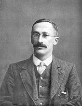
The term «t-statistic» is abbreviated from «hypothesis test statistic».[1] In statistics, the t-distribution was first derived as a posterior distribution in 1876 by Helmert[2][3][4] and Lüroth.[5][6][7] The t-distribution also appeared in a more general form as Pearson Type IV distribution in Karl Pearson’s 1895 paper.[8] However, the T-Distribution, also known as Student’s t-distribution, gets its name from William Sealy Gosset who first published it in English in 1908 in the scientific journal Biometrika using the pseudonym «Student»[9][10] because his employer preferred staff to use pen names when publishing scientific papers.[11] Gosset worked at the Guinness Brewery in Dublin, Ireland, and was interested in the problems of small samples – for example, the chemical properties of barley with small sample sizes. Hence a second version of the etymology of the term Student is that Guinness did not want their competitors to know that they were using the t-test to determine the quality of raw material (see Student’s t-distribution for a detailed history of this pseudonym, which is not to be confused with the literal term student). Although it was William Gosset after whom the term «Student» is penned, it was actually through the work of Ronald Fisher that the distribution became well known as «Student’s distribution»[12] and «Student’s t-test».
Gosset had been hired owing to Claude Guinness’s policy of recruiting the best graduates from Oxford and Cambridge to apply biochemistry and statistics to Guinness’s industrial processes.[13] Gosset devised the t-test as an economical way to monitor the quality of stout. The t-test work was submitted to and accepted in the journal Biometrika and published in 1908.[14]
Guinness had a policy of allowing technical staff leave for study (so-called «study leave»), which Gosset used during the first two terms of the 1906–1907 academic year in Professor Karl Pearson’s Biometric Laboratory at University College London.[15] Gosset’s identity was then known to fellow statisticians and to editor-in-chief Karl Pearson.[16]
Uses[edit]
The most frequently used t-tests are one-sample and two-sample tests:
- A one-sample location test of whether the mean of a population has a value specified in a null hypothesis.
- A two-sample location test of the null hypothesis such that the means of two populations are equal. All such tests are usually called Student’s t-tests, though strictly speaking that name should only be used if the variances of the two populations are also assumed to be equal; the form of the test used when this assumption is dropped is sometimes called Welch’s t-test. These tests are often referred to as unpaired or independent samples t-tests, as they are typically applied when the statistical units underlying the two samples being compared are non-overlapping.[17]
Assumptions[edit]
[dubious – discuss]
Most test statistics have the form t = Z/s, where Z and s are functions of the data.
Z may be sensitive to the alternative hypothesis (i.e., its magnitude tends to be larger when the alternative hypothesis is true), whereas s is a scaling parameter that allows the distribution of t to be determined.
As an example, in the one-sample t-test
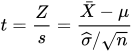
where X is the sample mean from a sample X1, X2, …, Xn, of size n, s is the standard error of the mean, 
The assumptions underlying a t-test in the simplest form above are that:
- X follows a normal distribution with mean μ and variance σ2/n
- s2(n − 1)/σ2 follows a χ2 distribution with n − 1 degrees of freedom. This assumption is met when the observations used for estimating s2 come from a normal distribution (and i.i.d for each group).
- Z and s are independent.
In the t-test comparing the means of two independent samples, the following assumptions should be met:
- The means of the two populations being compared should follow normal distributions. Under weak assumptions, this follows in large samples from the central limit theorem, even when the distribution of observations in each group is non-normal.[18]
- If using Student’s original definition of the t-test, the two populations being compared should have the same variance (testable using F-test, Levene’s test, Bartlett’s test, or the Brown–Forsythe test; or assessable graphically using a Q–Q plot). If the sample sizes in the two groups being compared are equal, Student’s original t-test is highly robust to the presence of unequal variances.[19] Welch’s t-test is insensitive to equality of the variances regardless of whether the sample sizes are similar.
- The data used to carry out the test should either be sampled independently from the two populations being compared or be fully paired. This is in general not testable from the data, but if the data are known to be dependent (e.g. paired by test design), a dependent test has to be applied. For partially paired data, the classical independent t-tests may give invalid results as the test statistic might not follow a t distribution, while the dependent t-test is sub-optimal as it discards the unpaired data.[20]
Most two-sample t-tests are robust to all but large deviations from the assumptions.[21]
For exactness, the t-test and Z-test require normality of the sample means, and the t-test additionally requires that the sample variance follows a scaled χ2 distribution, and that the sample mean and sample variance be statistically independent. Normality of the individual data values is not required if these conditions are met. By the central limit theorem, sample means of moderately large samples are often well-approximated by a normal distribution even if the data are not normally distributed. For non-normal data, the distribution of the sample variance may deviate substantially from a χ2 distribution.
However, if the sample size is large, Slutsky’s theorem implies that the distribution of the sample variance has little effect on the distribution of the test statistic. That is as sample size 
Unpaired and paired two-sample t-tests[edit]
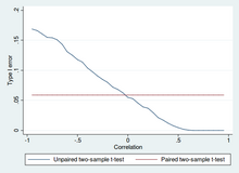
Type I error of unpaired and paired two-sample t-tests as a function of the correlation. The simulated random numbers originate from a bivariate normal distribution with a variance of 1. The significance level is 5% and the number of cases is 60.

Power of unpaired and paired two-sample t-tests as a function of the correlation. The simulated random numbers originate from a bivariate normal distribution with a variance of 1 and a deviation of the expected value of 0.4. The significance level is 5% and the number of cases is 60.
Two-sample t-tests for a difference in means involve independent samples (unpaired samples) or paired samples. Paired t-tests are a form of blocking, and have greater power (probability of avoiding a type II error, also known as a false negative) than unpaired tests when the paired units are similar with respect to «noise factors» that are independent of membership in the two groups being compared.[22] In a different context, paired t-tests can be used to reduce the effects of confounding factors in an observational study.
Independent (unpaired) samples[edit]
The independent samples t-test is used when two separate sets of independent and identically distributed samples are obtained, and one variable from each of the two populations is compared. For example, suppose we are evaluating the effect of a medical treatment, and we enroll 100 subjects into our study, then randomly assign 50 subjects to the treatment group and 50 subjects to the control group. In this case, we have two independent samples and would use the unpaired form of the t-test.
Paired samples[edit]
Paired samples t-tests typically consist of a sample of matched pairs of similar units, or one group of units that has been tested twice (a «repeated measures» t-test).
A typical example of the repeated measures t-test would be where subjects are tested prior to a treatment, say for high blood pressure, and the same subjects are tested again after treatment with a blood-pressure-lowering medication. By comparing the same patient’s numbers before and after treatment, we are effectively using each patient as their own control. That way the correct rejection of the null hypothesis (here: of no difference made by the treatment) can become much more likely, with statistical power increasing simply because the random interpatient variation has now been eliminated. However, an increase of statistical power comes at a price: more tests are required, each subject having to be tested twice. Because half of the sample now depends on the other half, the paired version of Student’s t-test has only n/2 − 1 degrees of freedom (with n being the total number of observations). Pairs become individual test units, and the sample has to be doubled to achieve the same number of degrees of freedom. Normally, there are n − 1 degrees of freedom (with n being the total number of observations).[23]
A paired samples t-test based on a «matched-pairs sample» results from an unpaired sample that is subsequently used to form a paired sample, by using additional variables that were measured along with the variable of interest.[24] The matching is carried out by identifying pairs of values consisting of one observation from each of the two samples, where the pair is similar in terms of other measured variables. This approach is sometimes used in observational studies to reduce or eliminate the effects of confounding factors.
Paired samples t-tests are often referred to as «dependent samples t-tests».
Calculations[edit]
Explicit expressions that can be used to carry out various t-tests are given below. In each case, the formula for a test statistic that either exactly follows or closely approximates a t-distribution under the null hypothesis is given. Also, the appropriate degrees of freedom are given in each case. Each of these statistics can be used to carry out either a one-tailed or two-tailed test.
Once the t value and degrees of freedom are determined, a p-value can be found using a table of values from Student’s t-distribution. If the calculated p-value is below the threshold chosen for statistical significance (usually the 0.10, the 0.05, or 0.01 level), then the null hypothesis is rejected in favor of the alternative hypothesis.
One-sample t-test[edit]
In testing the null hypothesis that the population mean is equal to a specified value μ0, one uses the statistic

where 
Although the parent population does not need to be normally distributed, the distribution of the population of sample means
By the central limit theorem, if the observations are independent and the second moment exists, then 
Slope of a regression line[edit]
Suppose one is fitting the model

where x is known, α and β are unknown, ε is a normally distributed random variable with mean 0 and unknown variance σ2, and Y is the outcome of interest. We want to test the null hypothesis that the slope β is equal to some specified value β0 (often taken to be 0, in which case the null hypothesis is that x and y are uncorrelated).
Let

Then
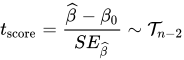
has a t-distribution with n − 2 degrees of freedom if the null hypothesis is true. The standard error of the slope coefficient:
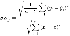
can be written in terms of the residuals. Let

Then tscore is given by:
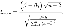
Another way to determine the tscore is:
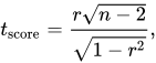
where r is the Pearson correlation coefficient.
The tscore, intercept can be determined from the tscore, slope:
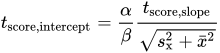
where sx2 is the sample variance.
Independent two-sample t-test[edit]
Equal sample sizes and variance[edit]
Given two groups (1, 2), this test is only applicable when:
- the two sample sizes are equal;
- it can be assumed that the two distributions have the same variance;
Violations of these assumptions are discussed below.
The t statistic to test whether the means are different can be calculated as follows:
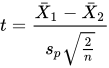
where
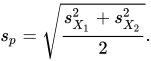
Here sp is the pooled standard deviation for n = n1 = n2 and s 2
X1 and s 2
X2 are the unbiased estimators of the population variance. The denominator of t is the standard error of the difference between two means.
For significance testing, the degrees of freedom for this test is 2n − 2 where n is sample size.
Equal or unequal sample sizes, similar variances (1/2 < sX1/sX2 < 2)[edit]
This test is used only when it can be assumed that the two distributions have the same variance. (When this assumption is violated, see below.)
The previous formulae are a special case of the formulae below, one recovers them when both samples are equal in size: n = n1 = n2.
The t statistic to test whether the means are different can be calculated as follows:
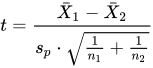
where
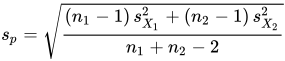
is the pooled standard deviation of the two samples: it is defined in this way so that its square is an unbiased estimator of the common variance whether or not the population means are the same. In these formulae, ni − 1 is the number of degrees of freedom for each group, and the total sample size minus two (that is, n1 + n2 − 2) is the total number of degrees of freedom, which is used in significance testing.
Equal or unequal sample sizes, unequal variances (sX1 > 2sX2 or sX2 > 2sX1)[edit]
This test, also known as Welch’s t-test, is used only when the two population variances are not assumed to be equal (the two sample sizes may or may not be equal) and hence must be estimated separately. The t statistic to test whether the population means are different is calculated as:
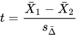
where
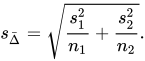
Here si2 is the unbiased estimator of the variance of each of the two samples with ni = number of participants in group i (i = 1 or 2). In this case
is not a pooled variance. For use in significance testing, the distribution of the test statistic is approximated as an ordinary Student’s t-distribution with the degrees of freedom calculated using

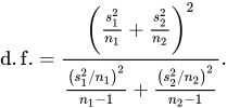
This is known as the Welch–Satterthwaite equation. The true distribution of the test statistic actually depends (slightly) on the two unknown population variances (see Behrens–Fisher problem).
Exact method for unequal variances and sample sizes[edit]
The test[25] deals with the famous Behrens–Fisher problem, i.e., comparing the difference between the means of two normally distributed populations when the variances of the two populations are not assumed to be equal, based on two independent samples.
The test is developed as an exact test that allows for unequal sample sizes and unequal variances of two populations. The exact property still holds even with small extremely small and unbalanced sample sizes (e.g. 
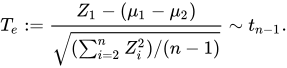
The Te statistic to test whether the means are different can be calculated as follows:
Let ![{displaystyle X=[X_{1},X_{2},ldots ,X_{m}]^{T}}](https://wikimedia.org/api/rest_v1/media/math/render/svg/a0f37f25b326e4b6229a7f0be5283ace07d1a97f)
![{displaystyle Y=[Y_{1},Y_{2},ldots ,Y_{n}]^{T}}](https://wikimedia.org/api/rest_v1/media/math/render/svg/a81b49d1f74f1a3c22759407966c63524eac1d2e)


Let 


Then 

From the above distribution we see that


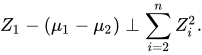
Dependent t-test for paired samples[edit]
This test is used when the samples are dependent; that is, when there is only one sample that has been tested twice (repeated measures) or when there are two samples that have been matched or «paired». This is an example of a paired difference test. The t statistic is calculated as
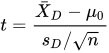
where 

-
Example of repeated measures
Number Name Test 1 Test 2 1 Mike 35% 67% 2 Melanie 50% 46% 3 Melissa 90% 86% 4 Mitchell 78% 91%
-
Example of matched pairs
Pair Name Age Test 1 John 35 250 1 Jane 36 340 2 Jimmy 22 460 2 Jessy 21 200
Worked examples[edit]
Let A1 denote a set obtained by drawing a random sample of six measurements:

and let A2 denote a second set obtained similarly:

These could be, for example, the weights of screws that were chosen out of a bucket.
We will carry out tests of the null hypothesis that the means of the populations from which the two samples were taken are equal.
The difference between the two sample means, each denoted by Xi, which appears in the numerator for all the two-sample testing approaches discussed above, is

The sample standard deviations for the two samples are approximately 0.05 and 0.11, respectively. For such small samples, a test of equality between the two population variances would not be very powerful. Since the sample sizes are equal, the two forms of the two-sample t-test will perform similarly in this example.
Unequal variances[edit]
If the approach for unequal variances (discussed above) is followed, the results are
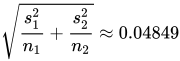
and the degrees of freedom

The test statistic is approximately 1.959, which gives a two-tailed test p-value of 0.09077.
Equal variances[edit]
If the approach for equal variances (discussed above) is followed, the results are
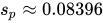
and the degrees of freedom

The test statistic is approximately equal to 1.959, which gives a two-tailed p-value of 0.07857.
[edit]
Alternatives to the t-test for location problems[edit]
The t-test provides an exact test for the equality of the means of two i.i.d. normal populations with unknown, but equal, variances. (Welch’s t-test is a nearly exact test for the case where the data are normal but the variances may differ.) For moderately large samples and a one tailed test, the t-test is relatively robust to moderate violations of the normality assumption.[26] In large enough samples, the t-test asymptotically approaches the z-test, and becomes robust even to large deviations from normality.[18]
If the data are substantially non-normal and the sample size is small, the t-test can give misleading results. See Location test for Gaussian scale mixture distributions for some theory related to one particular family of non-normal distributions.
When the normality assumption does not hold, a non-parametric alternative to the t-test may have better statistical power. However, when data are non-normal with differing variances between groups, a t-test may have better type-1 error control than some non-parametric alternatives.[27] Furthermore, non-parametric methods, such as the Mann-Whitney U test discussed below, typically do not test for a difference of means, so should be used carefully if a difference of means is of primary scientific interest.[18] For example, Mann-Whitney U test will keep the type 1 error at the desired level alpha if both groups have the same distribution. It will also have power in detecting an alternative by which group B has the same distribution as A but after some shift by a constant (in which case there would indeed be a difference in the means of the two groups). However, there could be cases where group A and B will have different distributions but with the same means (such as two distributions, one with positive skewness and the other with a negative one, but shifted so to have the same means). In such cases, MW could have more than alpha level power in rejecting the Null hypothesis but attributing the interpretation of difference in means to such a result would be incorrect.
In the presence of an outlier, the t-test is not robust. For example, for two independent samples when the data distributions are asymmetric (that is, the distributions are skewed) or the distributions have large tails, then the Wilcoxon rank-sum test (also known as the Mann–Whitney U test) can have three to four times higher power than the t-test.[26][28][29] The nonparametric counterpart to the paired samples t-test is the Wilcoxon signed-rank test for paired samples. For a discussion on choosing between the t-test and nonparametric alternatives, see Lumley, et al. (2002).[18]
One-way analysis of variance (ANOVA) generalizes the two-sample t-test when the data belong to more than two groups.
A design which includes both paired observations and independent observations[edit]
When both paired observations and independent observations are present in the two sample design, assuming data are missing completely at random (MCAR), the paired observations or independent observations may be discarded in order to proceed with the standard tests above. Alternatively making use of all of the available data, assuming normality and MCAR, the generalized partially overlapping samples t-test could be used.[30]
Multivariate testing[edit]
A generalization of Student’s t statistic, called Hotelling’s t-squared statistic, allows for the testing of hypotheses on multiple (often correlated) measures within the same sample. For instance, a researcher might submit a number of subjects to a personality test consisting of multiple personality scales (e.g. the Minnesota Multiphasic Personality Inventory). Because measures of this type are usually positively correlated, it is not advisable to conduct separate univariate t-tests to test hypotheses, as these would neglect the covariance among measures and inflate the chance of falsely rejecting at least one hypothesis (Type I error). In this case a single multivariate test is preferable for hypothesis testing. Fisher’s Method for combining multiple tests with alpha reduced for positive correlation among tests is one. Another is Hotelling’s T2 statistic follows a T2 distribution. However, in practice the distribution is rarely used, since tabulated values for T2 are hard to find. Usually, T2 is converted instead to an F statistic.
For a one-sample multivariate test, the hypothesis is that the mean vector (μ) is equal to a given vector (μ0). The test statistic is Hotelling’s t2:

where n is the sample size, x is the vector of column means and S is an m × m sample covariance matrix.
For a two-sample multivariate test, the hypothesis is that the mean vectors (μ1, μ2) of two samples are equal. The test statistic is Hotelling’s two-sample t2:

Software implementations[edit]
Many spreadsheet programs and statistics packages, such as QtiPlot, LibreOffice Calc, Microsoft Excel, SAS, SPSS, Stata, DAP, gretl, R, Python, PSPP, MATLAB and Minitab, include implementations of Student’s t-test.
| Language/Program | Function | Notes |
|---|---|---|
| Microsoft Excel pre 2010 | TTEST(array1, array2, tails, type) |
See [1] |
| Microsoft Excel 2010 and later | T.TEST(array1, array2, tails, type) |
See [2] |
| Apple Numbers | TTEST(sample-1-values, sample-2-values, tails, test-type) |
See [3] |
| LibreOffice Calc | TTEST(Data1; Data2; Mode; Type) |
See [4] |
| Google Sheets | TTEST(range1, range2, tails, type) |
See [5] |
| Python | scipy.stats.ttest_ind(a, b, equal_var=True) |
See [6] |
| MATLAB | ttest(data1, data2) |
See [7] |
| Mathematica | TTest[{data1,data2}] |
See [8] |
| R | t.test(data1, data2, var.equal=TRUE) |
See [9] |
| SAS | PROC TTEST |
See [10] |
| Java | tTest(sample1, sample2) |
See [11] |
| Julia | EqualVarianceTTest(sample1, sample2) |
See [12] |
| Stata | ttest data1 == data2 |
See [13] |
See also[edit]
- Conditional change model
- F-test
- Noncentral t-distribution in power analysis
- Student’s t-statistic
- Z-test
- Mann–Whitney U test
- Šidák correction for t-test
- Welch’s t-test
- Analysis of variance (ANOVA)
References[edit]
Citations[edit]
- ^ The Microbiome in Health and Disease. Academic Press. 2020-05-29. p. 397. ISBN 978-0-12-820001-8.
- ^ Szabó, István (2003), «Systeme aus einer endlichen Anzahl starrer Körper», Einführung in die Technische Mechanik, Springer Berlin Heidelberg, pp. 196–199, doi:10.1007/978-3-642-61925-0_16, ISBN 978-3-540-13293-6
- ^ Schlyvitch, B. (October 1937). «Untersuchungen über den anastomotischen Kanal zwischen der Arteria coeliaca und mesenterica superior und damit in Zusammenhang stehende Fragen». Zeitschrift für Anatomie und Entwicklungsgeschichte. 107 (6): 709–737. doi:10.1007/bf02118337. ISSN 0340-2061. S2CID 27311567.
- ^ Helmert (1876). «Die Genauigkeit der Formel von Peters zur Berechnung des wahrscheinlichen Beobachtungsfehlers directer Beobachtungen gleicher Genauigkeit». Astronomische Nachrichten (in German). 88 (8–9): 113–131. Bibcode:1876AN…..88..113H. doi:10.1002/asna.18760880802.
- ^ Lüroth, J. (1876). «Vergleichung von zwei Werthen des wahrscheinlichen Fehlers». Astronomische Nachrichten (in German). 87 (14): 209–220. Bibcode:1876AN…..87..209L. doi:10.1002/asna.18760871402.
- ^ Pfanzagl J, Sheynin O (1996). «Studies in the history of probability and statistics. XLIV. A forerunner of the t-distribution». Biometrika. 83 (4): 891–898. doi:10.1093/biomet/83.4.891. MR 1766040.
- ^ Sheynin, Oscar (1995). «Helmert’s work in the theory of errors». Archive for History of Exact Sciences. 49 (1): 73–104. doi:10.1007/BF00374700. ISSN 0003-9519. S2CID 121241599.
- ^ Pearson, K. (1895-01-01). «Contributions to the Mathematical Theory of Evolution. II. Skew Variation in Homogeneous Material». Philosophical Transactions of the Royal Society A: Mathematical, Physical and Engineering Sciences. 186: 343–414 (374). doi:10.1098/rsta.1895.0010. ISSN 1364-503X
- ^ «Student» William Sealy Gosset (1908). «The probable error of a mean» (PDF). Biometrika. 6 (1): 1–25. doi:10.1093/biomet/6.1.1. hdl:10338.dmlcz/143545. JSTOR 2331554
- ^ «T Table».
- ^ Wendl MC (2016). «Pseudonymous fame». Science. 351 (6280): 1406. doi:10.1126/science.351.6280.1406. PMID 27013722
- ^ Walpole, Ronald E. (2006). Probability & statistics for engineers & scientists. Myers, H. Raymond. (7th ed.). New Delhi: Pearson. ISBN 81-7758-404-9. OCLC 818811849.
- ^ O’Connor, John J.; Robertson, Edmund F., «William Sealy Gosset», MacTutor History of Mathematics archive, University of St Andrews
- ^ «The Probable Error of a Mean» (PDF). Biometrika. 6 (1): 1–25. 1908. doi:10.1093/biomet/6.1.1. hdl:10338.dmlcz/143545. Retrieved 24 July 2016.
- ^ Raju, T. N. (2005). «William Sealy Gosset and William A. Silverman: Two ‘Students’ of Science». Pediatrics. 116 (3): 732–5. doi:10.1542/peds.2005-1134. PMID 16140715. S2CID 32745754.
- ^ Dodge, Yadolah (2008). The Concise Encyclopedia of Statistics. Springer Science & Business Media. pp. 234–235. ISBN 978-0-387-31742-7.
- ^ Fadem, Barbara (2008). High-Yield Behavioral Science. High-Yield Series. Hagerstown, MD: Lippincott Williams & Wilkins. ISBN 9781451130300.
- ^ a b c d Lumley, Thomas; Diehr, Paula; Emerson, Scott; Chen, Lu (May 2002). «The Importance of the Normality Assumption in Large Public Health Data Sets». Annual Review of Public Health. 23 (1): 151–169. doi:10.1146/annurev.publhealth.23.100901.140546. ISSN 0163-7525. PMID 11910059.
- ^ Markowski, Carol A.; Markowski, Edward P. (1990). «Conditions for the Effectiveness of a Preliminary Test of Variance». The American Statistician. 44 (4): 322–326. doi:10.2307/2684360. JSTOR 2684360.
- ^ Guo, Beibei; Yuan, Ying (2017). «A comparative review of methods for comparing means using partially paired data». Statistical Methods in Medical Research. 26 (3): 1323–1340. doi:10.1177/0962280215577111. PMID 25834090. S2CID 46598415.
- ^ Bland, Martin (1995). An Introduction to Medical Statistics. Oxford University Press. p. 168. ISBN 978-0-19-262428-4.
- ^ Rice, John A. (2006). Mathematical Statistics and Data Analysis (3rd ed.). Duxbury Advanced.[ISBN missing]
- ^ Weisstein, Eric. «Student’s t-Distribution». mathworld.wolfram.com.
- ^ David, H. A.; Gunnink, Jason L. (1997). «The Paired t Test Under Artificial Pairing». The American Statistician. 51 (1): 9–12. doi:10.2307/2684684. JSTOR 2684684.
- ^ Chang Wang, Jinzhu Jia. «A New Non-asymptotic t-test for Behrens-Fisher Problems».https://arxiv.org/abs/2210.16473
- ^ a b Sawilowsky, Shlomo S.; Blair, R. Clifford (1992). «A More Realistic Look at the Robustness and Type II Error Properties of the t Test to Departures From Population Normality». Psychological Bulletin. 111 (2): 352–360. doi:10.1037/0033-2909.111.2.352.
- ^ Zimmerman, Donald W. (January 1998). «Invalidation of Parametric and Nonparametric Statistical Tests by Concurrent Violation of Two Assumptions». The Journal of Experimental Education. 67 (1): 55–68. doi:10.1080/00220979809598344. ISSN 0022-0973.
- ^ Blair, R. Clifford; Higgins, James J. (1980). «A Comparison of the Power of Wilcoxon’s Rank-Sum Statistic to That of Student’s t Statistic Under Various Nonnormal Distributions». Journal of Educational Statistics. 5 (4): 309–335. doi:10.2307/1164905. JSTOR 1164905.
- ^ Fay, Michael P.; Proschan, Michael A. (2010). «Wilcoxon–Mann–Whitney or t-test? On assumptions for hypothesis tests and multiple interpretations of decision rules». Statistics Surveys. 4: 1–39. doi:10.1214/09-SS051. PMC 2857732. PMID 20414472.
- ^ Derrick, B; Toher, D; White, P (2017). «How to compare the means of two samples that include paired observations and independent observations: A companion to Derrick, Russ, Toher and White (2017)» (PDF). The Quantitative Methods for Psychology. 13 (2): 120–126. doi:10.20982/tqmp.13.2.p120.
Sources[edit]
- O’Mahony, Michael (1986). Sensory Evaluation of Food: Statistical Methods and Procedures. CRC Press. p. 487. ISBN 0-82477337-3.
- Press, William H.; Teukolsky, Saul A.; Vetterling, William T.; Flannery, Brian P. (1992). Numerical Recipes in C: The Art of Scientific Computing. Cambridge University Press. p. 616. ISBN 0-521-43108-5.
Further reading[edit]
- Boneau, C. Alan (1960). «The effects of violations of assumptions underlying the t test». Psychological Bulletin. 57 (1): 49–64. doi:10.1037/h0041412. PMID 13802482.
- Edgell, Stephen E.; Noon, Sheila M. (1984). «Effect of violation of normality on the t test of the correlation coefficient». Psychological Bulletin. 95 (3): 576–583. doi:10.1037/0033-2909.95.3.576.
External links[edit]

Wikiversity has learning resources about t-test
- «Student test», Encyclopedia of Mathematics, EMS Press, 2001 [1994]
- Trochim, William M.K. «The T-Test», Research Methods Knowledge Base, conjoint.ly
- Econometrics lecture (topic: hypothesis testing) on YouTube by Mark Thoma
A t-test is any statistical hypothesis test in which the test statistic follows a Student’s t-distribution under the null hypothesis. It is most commonly applied when the test statistic would follow a normal distribution if the value of a scaling term in the test statistic were known (typically, the scaling term is unknown and therefore a nuisance parameter). When the scaling term is estimated based on the data, the test statistic—under certain conditions—follows a Student’s t distribution. The t-test’s most common application is to test whether the means of two populations are different.
History[edit]
The term «t-statistic» is abbreviated from «hypothesis test statistic».[1] In statistics, the t-distribution was first derived as a posterior distribution in 1876 by Helmert[2][3][4] and Lüroth.[5][6][7] The t-distribution also appeared in a more general form as Pearson Type IV distribution in Karl Pearson’s 1895 paper.[8] However, the T-Distribution, also known as Student’s t-distribution, gets its name from William Sealy Gosset who first published it in English in 1908 in the scientific journal Biometrika using the pseudonym «Student»[9][10] because his employer preferred staff to use pen names when publishing scientific papers.[11] Gosset worked at the Guinness Brewery in Dublin, Ireland, and was interested in the problems of small samples – for example, the chemical properties of barley with small sample sizes. Hence a second version of the etymology of the term Student is that Guinness did not want their competitors to know that they were using the t-test to determine the quality of raw material (see Student’s t-distribution for a detailed history of this pseudonym, which is not to be confused with the literal term student). Although it was William Gosset after whom the term «Student» is penned, it was actually through the work of Ronald Fisher that the distribution became well known as «Student’s distribution»[12] and «Student’s t-test».
Gosset had been hired owing to Claude Guinness’s policy of recruiting the best graduates from Oxford and Cambridge to apply biochemistry and statistics to Guinness’s industrial processes.[13] Gosset devised the t-test as an economical way to monitor the quality of stout. The t-test work was submitted to and accepted in the journal Biometrika and published in 1908.[14]
Guinness had a policy of allowing technical staff leave for study (so-called «study leave»), which Gosset used during the first two terms of the 1906–1907 academic year in Professor Karl Pearson’s Biometric Laboratory at University College London.[15] Gosset’s identity was then known to fellow statisticians and to editor-in-chief Karl Pearson.[16]
Uses[edit]
The most frequently used t-tests are one-sample and two-sample tests:
- A one-sample location test of whether the mean of a population has a value specified in a null hypothesis.
- A two-sample location test of the null hypothesis such that the means of two populations are equal. All such tests are usually called Student’s t-tests, though strictly speaking that name should only be used if the variances of the two populations are also assumed to be equal; the form of the test used when this assumption is dropped is sometimes called Welch’s t-test. These tests are often referred to as unpaired or independent samples t-tests, as they are typically applied when the statistical units underlying the two samples being compared are non-overlapping.[17]
Assumptions[edit]
[dubious – discuss]
Most test statistics have the form t = Z/s, where Z and s are functions of the data.
Z may be sensitive to the alternative hypothesis (i.e., its magnitude tends to be larger when the alternative hypothesis is true), whereas s is a scaling parameter that allows the distribution of t to be determined.
As an example, in the one-sample t-test
where X is the sample mean from a sample X1, X2, …, Xn, of size n, s is the standard error of the mean,
The assumptions underlying a t-test in the simplest form above are that:
- X follows a normal distribution with mean μ and variance σ2/n
- s2(n − 1)/σ2 follows a χ2 distribution with n − 1 degrees of freedom. This assumption is met when the observations used for estimating s2 come from a normal distribution (and i.i.d for each group).
- Z and s are independent.
In the t-test comparing the means of two independent samples, the following assumptions should be met:
- The means of the two populations being compared should follow normal distributions. Under weak assumptions, this follows in large samples from the central limit theorem, even when the distribution of observations in each group is non-normal.[18]
- If using Student’s original definition of the t-test, the two populations being compared should have the same variance (testable using F-test, Levene’s test, Bartlett’s test, or the Brown–Forsythe test; or assessable graphically using a Q–Q plot). If the sample sizes in the two groups being compared are equal, Student’s original t-test is highly robust to the presence of unequal variances.[19] Welch’s t-test is insensitive to equality of the variances regardless of whether the sample sizes are similar.
- The data used to carry out the test should either be sampled independently from the two populations being compared or be fully paired. This is in general not testable from the data, but if the data are known to be dependent (e.g. paired by test design), a dependent test has to be applied. For partially paired data, the classical independent t-tests may give invalid results as the test statistic might not follow a t distribution, while the dependent t-test is sub-optimal as it discards the unpaired data.[20]
Most two-sample t-tests are robust to all but large deviations from the assumptions.[21]
For exactness, the t-test and Z-test require normality of the sample means, and the t-test additionally requires that the sample variance follows a scaled χ2 distribution, and that the sample mean and sample variance be statistically independent. Normality of the individual data values is not required if these conditions are met. By the central limit theorem, sample means of moderately large samples are often well-approximated by a normal distribution even if the data are not normally distributed. For non-normal data, the distribution of the sample variance may deviate substantially from a χ2 distribution.
However, if the sample size is large, Slutsky’s theorem implies that the distribution of the sample variance has little effect on the distribution of the test statistic. That is as sample size
Unpaired and paired two-sample t-tests[edit]
Type I error of unpaired and paired two-sample t-tests as a function of the correlation. The simulated random numbers originate from a bivariate normal distribution with a variance of 1. The significance level is 5% and the number of cases is 60.
Power of unpaired and paired two-sample t-tests as a function of the correlation. The simulated random numbers originate from a bivariate normal distribution with a variance of 1 and a deviation of the expected value of 0.4. The significance level is 5% and the number of cases is 60.
Two-sample t-tests for a difference in means involve independent samples (unpaired samples) or paired samples. Paired t-tests are a form of blocking, and have greater power (probability of avoiding a type II error, also known as a false negative) than unpaired tests when the paired units are similar with respect to «noise factors» that are independent of membership in the two groups being compared.[22] In a different context, paired t-tests can be used to reduce the effects of confounding factors in an observational study.
Independent (unpaired) samples[edit]
The independent samples t-test is used when two separate sets of independent and identically distributed samples are obtained, and one variable from each of the two populations is compared. For example, suppose we are evaluating the effect of a medical treatment, and we enroll 100 subjects into our study, then randomly assign 50 subjects to the treatment group and 50 subjects to the control group. In this case, we have two independent samples and would use the unpaired form of the t-test.
Paired samples[edit]
Paired samples t-tests typically consist of a sample of matched pairs of similar units, or one group of units that has been tested twice (a «repeated measures» t-test).
A typical example of the repeated measures t-test would be where subjects are tested prior to a treatment, say for high blood pressure, and the same subjects are tested again after treatment with a blood-pressure-lowering medication. By comparing the same patient’s numbers before and after treatment, we are effectively using each patient as their own control. That way the correct rejection of the null hypothesis (here: of no difference made by the treatment) can become much more likely, with statistical power increasing simply because the random interpatient variation has now been eliminated. However, an increase of statistical power comes at a price: more tests are required, each subject having to be tested twice. Because half of the sample now depends on the other half, the paired version of Student’s t-test has only n/2 − 1 degrees of freedom (with n being the total number of observations). Pairs become individual test units, and the sample has to be doubled to achieve the same number of degrees of freedom. Normally, there are n − 1 degrees of freedom (with n being the total number of observations).[23]
A paired samples t-test based on a «matched-pairs sample» results from an unpaired sample that is subsequently used to form a paired sample, by using additional variables that were measured along with the variable of interest.[24] The matching is carried out by identifying pairs of values consisting of one observation from each of the two samples, where the pair is similar in terms of other measured variables. This approach is sometimes used in observational studies to reduce or eliminate the effects of confounding factors.
Paired samples t-tests are often referred to as «dependent samples t-tests».
Calculations[edit]
Explicit expressions that can be used to carry out various t-tests are given below. In each case, the formula for a test statistic that either exactly follows or closely approximates a t-distribution under the null hypothesis is given. Also, the appropriate degrees of freedom are given in each case. Each of these statistics can be used to carry out either a one-tailed or two-tailed test.
Once the t value and degrees of freedom are determined, a p-value can be found using a table of values from Student’s t-distribution. If the calculated p-value is below the threshold chosen for statistical significance (usually the 0.10, the 0.05, or 0.01 level), then the null hypothesis is rejected in favor of the alternative hypothesis.
One-sample t-test[edit]
In testing the null hypothesis that the population mean is equal to a specified value μ0, one uses the statistic
where
Although the parent population does not need to be normally distributed, the distribution of the population of sample means
By the central limit theorem, if the observations are independent and the second moment exists, then
Slope of a regression line[edit]
Suppose one is fitting the model
where x is known, α and β are unknown, ε is a normally distributed random variable with mean 0 and unknown variance σ2, and Y is the outcome of interest. We want to test the null hypothesis that the slope β is equal to some specified value β0 (often taken to be 0, in which case the null hypothesis is that x and y are uncorrelated).
Let
Then
has a t-distribution with n − 2 degrees of freedom if the null hypothesis is true. The standard error of the slope coefficient:
can be written in terms of the residuals. Let
Then tscore is given by:
Another way to determine the tscore is:
where r is the Pearson correlation coefficient.
The tscore, intercept can be determined from the tscore, slope:
where sx2 is the sample variance.
Independent two-sample t-test[edit]
Equal sample sizes and variance[edit]
Given two groups (1, 2), this test is only applicable when:
- the two sample sizes are equal;
- it can be assumed that the two distributions have the same variance;
Violations of these assumptions are discussed below.
The t statistic to test whether the means are different can be calculated as follows:
where
Here sp is the pooled standard deviation for n = n1 = n2 and s 2
X1 and s 2
X2 are the unbiased estimators of the population variance. The denominator of t is the standard error of the difference between two means.
For significance testing, the degrees of freedom for this test is 2n − 2 where n is sample size.
Equal or unequal sample sizes, similar variances (1/2 < sX1/sX2 < 2)[edit]
This test is used only when it can be assumed that the two distributions have the same variance. (When this assumption is violated, see below.)
The previous formulae are a special case of the formulae below, one recovers them when both samples are equal in size: n = n1 = n2.
The t statistic to test whether the means are different can be calculated as follows:
where
is the pooled standard deviation of the two samples: it is defined in this way so that its square is an unbiased estimator of the common variance whether or not the population means are the same. In these formulae, ni − 1 is the number of degrees of freedom for each group, and the total sample size minus two (that is, n1 + n2 − 2) is the total number of degrees of freedom, which is used in significance testing.
Equal or unequal sample sizes, unequal variances (sX1 > 2sX2 or sX2 > 2sX1)[edit]
This test, also known as Welch’s t-test, is used only when the two population variances are not assumed to be equal (the two sample sizes may or may not be equal) and hence must be estimated separately. The t statistic to test whether the population means are different is calculated as:
where
Here si2 is the unbiased estimator of the variance of each of the two samples with ni = number of participants in group i (i = 1 or 2). In this case
is not a pooled variance. For use in significance testing, the distribution of the test statistic is approximated as an ordinary Student’s t-distribution with the degrees of freedom calculated using
This is known as the Welch–Satterthwaite equation. The true distribution of the test statistic actually depends (slightly) on the two unknown population variances (see Behrens–Fisher problem).
Exact method for unequal variances and sample sizes[edit]
The test[25] deals with the famous Behrens–Fisher problem, i.e., comparing the difference between the means of two normally distributed populations when the variances of the two populations are not assumed to be equal, based on two independent samples.
The test is developed as an exact test that allows for unequal sample sizes and unequal variances of two populations. The exact property still holds even with small extremely small and unbalanced sample sizes (e.g.
The Te statistic to test whether the means are different can be calculated as follows:
Let
Let
Then
From the above distribution we see that
Dependent t-test for paired samples[edit]
This test is used when the samples are dependent; that is, when there is only one sample that has been tested twice (repeated measures) or when there are two samples that have been matched or «paired». This is an example of a paired difference test. The t statistic is calculated as
where
-
Example of repeated measures
Number Name Test 1 Test 2 1 Mike 35% 67% 2 Melanie 50% 46% 3 Melissa 90% 86% 4 Mitchell 78% 91%
-
Example of matched pairs
Pair Name Age Test 1 John 35 250 1 Jane 36 340 2 Jimmy 22 460 2 Jessy 21 200
Worked examples[edit]
Let A1 denote a set obtained by drawing a random sample of six measurements:
and let A2 denote a second set obtained similarly:
These could be, for example, the weights of screws that were chosen out of a bucket.
We will carry out tests of the null hypothesis that the means of the populations from which the two samples were taken are equal.
The difference between the two sample means, each denoted by Xi, which appears in the numerator for all the two-sample testing approaches discussed above, is
The sample standard deviations for the two samples are approximately 0.05 and 0.11, respectively. For such small samples, a test of equality between the two population variances would not be very powerful. Since the sample sizes are equal, the two forms of the two-sample t-test will perform similarly in this example.
Unequal variances[edit]
If the approach for unequal variances (discussed above) is followed, the results are
and the degrees of freedom
The test statistic is approximately 1.959, which gives a two-tailed test p-value of 0.09077.
Equal variances[edit]
If the approach for equal variances (discussed above) is followed, the results are
and the degrees of freedom
The test statistic is approximately equal to 1.959, which gives a two-tailed p-value of 0.07857.
[edit]
Alternatives to the t-test for location problems[edit]
The t-test provides an exact test for the equality of the means of two i.i.d. normal populations with unknown, but equal, variances. (Welch’s t-test is a nearly exact test for the case where the data are normal but the variances may differ.) For moderately large samples and a one tailed test, the t-test is relatively robust to moderate violations of the normality assumption.[26] In large enough samples, the t-test asymptotically approaches the z-test, and becomes robust even to large deviations from normality.[18]
If the data are substantially non-normal and the sample size is small, the t-test can give misleading results. See Location test for Gaussian scale mixture distributions for some theory related to one particular family of non-normal distributions.
When the normality assumption does not hold, a non-parametric alternative to the t-test may have better statistical power. However, when data are non-normal with differing variances between groups, a t-test may have better type-1 error control than some non-parametric alternatives.[27] Furthermore, non-parametric methods, such as the Mann-Whitney U test discussed below, typically do not test for a difference of means, so should be used carefully if a difference of means is of primary scientific interest.[18] For example, Mann-Whitney U test will keep the type 1 error at the desired level alpha if both groups have the same distribution. It will also have power in detecting an alternative by which group B has the same distribution as A but after some shift by a constant (in which case there would indeed be a difference in the means of the two groups). However, there could be cases where group A and B will have different distributions but with the same means (such as two distributions, one with positive skewness and the other with a negative one, but shifted so to have the same means). In such cases, MW could have more than alpha level power in rejecting the Null hypothesis but attributing the interpretation of difference in means to such a result would be incorrect.
In the presence of an outlier, the t-test is not robust. For example, for two independent samples when the data distributions are asymmetric (that is, the distributions are skewed) or the distributions have large tails, then the Wilcoxon rank-sum test (also known as the Mann–Whitney U test) can have three to four times higher power than the t-test.[26][28][29] The nonparametric counterpart to the paired samples t-test is the Wilcoxon signed-rank test for paired samples. For a discussion on choosing between the t-test and nonparametric alternatives, see Lumley, et al. (2002).[18]
One-way analysis of variance (ANOVA) generalizes the two-sample t-test when the data belong to more than two groups.
A design which includes both paired observations and independent observations[edit]
When both paired observations and independent observations are present in the two sample design, assuming data are missing completely at random (MCAR), the paired observations or independent observations may be discarded in order to proceed with the standard tests above. Alternatively making use of all of the available data, assuming normality and MCAR, the generalized partially overlapping samples t-test could be used.[30]
Multivariate testing[edit]
A generalization of Student’s t statistic, called Hotelling’s t-squared statistic, allows for the testing of hypotheses on multiple (often correlated) measures within the same sample. For instance, a researcher might submit a number of subjects to a personality test consisting of multiple personality scales (e.g. the Minnesota Multiphasic Personality Inventory). Because measures of this type are usually positively correlated, it is not advisable to conduct separate univariate t-tests to test hypotheses, as these would neglect the covariance among measures and inflate the chance of falsely rejecting at least one hypothesis (Type I error). In this case a single multivariate test is preferable for hypothesis testing. Fisher’s Method for combining multiple tests with alpha reduced for positive correlation among tests is one. Another is Hotelling’s T2 statistic follows a T2 distribution. However, in practice the distribution is rarely used, since tabulated values for T2 are hard to find. Usually, T2 is converted instead to an F statistic.
For a one-sample multivariate test, the hypothesis is that the mean vector (μ) is equal to a given vector (μ0). The test statistic is Hotelling’s t2:
where n is the sample size, x is the vector of column means and S is an m × m sample covariance matrix.
For a two-sample multivariate test, the hypothesis is that the mean vectors (μ1, μ2) of two samples are equal. The test statistic is Hotelling’s two-sample t2:
Software implementations[edit]
Many spreadsheet programs and statistics packages, such as QtiPlot, LibreOffice Calc, Microsoft Excel, SAS, SPSS, Stata, DAP, gretl, R, Python, PSPP, MATLAB and Minitab, include implementations of Student’s t-test.
| Language/Program | Function | Notes |
|---|---|---|
| Microsoft Excel pre 2010 | TTEST(array1, array2, tails, type) |
See [1] |
| Microsoft Excel 2010 and later | T.TEST(array1, array2, tails, type) |
See [2] |
| Apple Numbers | TTEST(sample-1-values, sample-2-values, tails, test-type) |
See [3] |
| LibreOffice Calc | TTEST(Data1; Data2; Mode; Type) |
See [4] |
| Google Sheets | TTEST(range1, range2, tails, type) |
See [5] |
| Python | scipy.stats.ttest_ind(a, b, equal_var=True) |
See [6] |
| MATLAB | ttest(data1, data2) |
See [7] |
| Mathematica | TTest[{data1,data2}] |
See [8] |
| R | t.test(data1, data2, var.equal=TRUE) |
See [9] |
| SAS | PROC TTEST |
See [10] |
| Java | tTest(sample1, sample2) |
See [11] |
| Julia | EqualVarianceTTest(sample1, sample2) |
See [12] |
| Stata | ttest data1 == data2 |
See [13] |
See also[edit]
- Conditional change model
- F-test
- Noncentral t-distribution in power analysis
- Student’s t-statistic
- Z-test
- Mann–Whitney U test
- Šidák correction for t-test
- Welch’s t-test
- Analysis of variance (ANOVA)
References[edit]
Citations[edit]
- ^ The Microbiome in Health and Disease. Academic Press. 2020-05-29. p. 397. ISBN 978-0-12-820001-8.
- ^ Szabó, István (2003), «Systeme aus einer endlichen Anzahl starrer Körper», Einführung in die Technische Mechanik, Springer Berlin Heidelberg, pp. 196–199, doi:10.1007/978-3-642-61925-0_16, ISBN 978-3-540-13293-6
- ^ Schlyvitch, B. (October 1937). «Untersuchungen über den anastomotischen Kanal zwischen der Arteria coeliaca und mesenterica superior und damit in Zusammenhang stehende Fragen». Zeitschrift für Anatomie und Entwicklungsgeschichte. 107 (6): 709–737. doi:10.1007/bf02118337. ISSN 0340-2061. S2CID 27311567.
- ^ Helmert (1876). «Die Genauigkeit der Formel von Peters zur Berechnung des wahrscheinlichen Beobachtungsfehlers directer Beobachtungen gleicher Genauigkeit». Astronomische Nachrichten (in German). 88 (8–9): 113–131. Bibcode:1876AN…..88..113H. doi:10.1002/asna.18760880802.
- ^ Lüroth, J. (1876). «Vergleichung von zwei Werthen des wahrscheinlichen Fehlers». Astronomische Nachrichten (in German). 87 (14): 209–220. Bibcode:1876AN…..87..209L. doi:10.1002/asna.18760871402.
- ^ Pfanzagl J, Sheynin O (1996). «Studies in the history of probability and statistics. XLIV. A forerunner of the t-distribution». Biometrika. 83 (4): 891–898. doi:10.1093/biomet/83.4.891. MR 1766040.
- ^ Sheynin, Oscar (1995). «Helmert’s work in the theory of errors». Archive for History of Exact Sciences. 49 (1): 73–104. doi:10.1007/BF00374700. ISSN 0003-9519. S2CID 121241599.
- ^ Pearson, K. (1895-01-01). «Contributions to the Mathematical Theory of Evolution. II. Skew Variation in Homogeneous Material». Philosophical Transactions of the Royal Society A: Mathematical, Physical and Engineering Sciences. 186: 343–414 (374). doi:10.1098/rsta.1895.0010. ISSN 1364-503X
- ^ «Student» William Sealy Gosset (1908). «The probable error of a mean» (PDF). Biometrika. 6 (1): 1–25. doi:10.1093/biomet/6.1.1. hdl:10338.dmlcz/143545. JSTOR 2331554
- ^ «T Table».
- ^ Wendl MC (2016). «Pseudonymous fame». Science. 351 (6280): 1406. doi:10.1126/science.351.6280.1406. PMID 27013722
- ^ Walpole, Ronald E. (2006). Probability & statistics for engineers & scientists. Myers, H. Raymond. (7th ed.). New Delhi: Pearson. ISBN 81-7758-404-9. OCLC 818811849.
- ^ O’Connor, John J.; Robertson, Edmund F., «William Sealy Gosset», MacTutor History of Mathematics archive, University of St Andrews
- ^ «The Probable Error of a Mean» (PDF). Biometrika. 6 (1): 1–25. 1908. doi:10.1093/biomet/6.1.1. hdl:10338.dmlcz/143545. Retrieved 24 July 2016.
- ^ Raju, T. N. (2005). «William Sealy Gosset and William A. Silverman: Two ‘Students’ of Science». Pediatrics. 116 (3): 732–5. doi:10.1542/peds.2005-1134. PMID 16140715. S2CID 32745754.
- ^ Dodge, Yadolah (2008). The Concise Encyclopedia of Statistics. Springer Science & Business Media. pp. 234–235. ISBN 978-0-387-31742-7.
- ^ Fadem, Barbara (2008). High-Yield Behavioral Science. High-Yield Series. Hagerstown, MD: Lippincott Williams & Wilkins. ISBN 9781451130300.
- ^ a b c d Lumley, Thomas; Diehr, Paula; Emerson, Scott; Chen, Lu (May 2002). «The Importance of the Normality Assumption in Large Public Health Data Sets». Annual Review of Public Health. 23 (1): 151–169. doi:10.1146/annurev.publhealth.23.100901.140546. ISSN 0163-7525. PMID 11910059.
- ^ Markowski, Carol A.; Markowski, Edward P. (1990). «Conditions for the Effectiveness of a Preliminary Test of Variance». The American Statistician. 44 (4): 322–326. doi:10.2307/2684360. JSTOR 2684360.
- ^ Guo, Beibei; Yuan, Ying (2017). «A comparative review of methods for comparing means using partially paired data». Statistical Methods in Medical Research. 26 (3): 1323–1340. doi:10.1177/0962280215577111. PMID 25834090. S2CID 46598415.
- ^ Bland, Martin (1995). An Introduction to Medical Statistics. Oxford University Press. p. 168. ISBN 978-0-19-262428-4.
- ^ Rice, John A. (2006). Mathematical Statistics and Data Analysis (3rd ed.). Duxbury Advanced.[ISBN missing]
- ^ Weisstein, Eric. «Student’s t-Distribution». mathworld.wolfram.com.
- ^ David, H. A.; Gunnink, Jason L. (1997). «The Paired t Test Under Artificial Pairing». The American Statistician. 51 (1): 9–12. doi:10.2307/2684684. JSTOR 2684684.
- ^ Chang Wang, Jinzhu Jia. «A New Non-asymptotic t-test for Behrens-Fisher Problems».https://arxiv.org/abs/2210.16473
- ^ a b Sawilowsky, Shlomo S.; Blair, R. Clifford (1992). «A More Realistic Look at the Robustness and Type II Error Properties of the t Test to Departures From Population Normality». Psychological Bulletin. 111 (2): 352–360. doi:10.1037/0033-2909.111.2.352.
- ^ Zimmerman, Donald W. (January 1998). «Invalidation of Parametric and Nonparametric Statistical Tests by Concurrent Violation of Two Assumptions». The Journal of Experimental Education. 67 (1): 55–68. doi:10.1080/00220979809598344. ISSN 0022-0973.
- ^ Blair, R. Clifford; Higgins, James J. (1980). «A Comparison of the Power of Wilcoxon’s Rank-Sum Statistic to That of Student’s t Statistic Under Various Nonnormal Distributions». Journal of Educational Statistics. 5 (4): 309–335. doi:10.2307/1164905. JSTOR 1164905.
- ^ Fay, Michael P.; Proschan, Michael A. (2010). «Wilcoxon–Mann–Whitney or t-test? On assumptions for hypothesis tests and multiple interpretations of decision rules». Statistics Surveys. 4: 1–39. doi:10.1214/09-SS051. PMC 2857732. PMID 20414472.
- ^ Derrick, B; Toher, D; White, P (2017). «How to compare the means of two samples that include paired observations and independent observations: A companion to Derrick, Russ, Toher and White (2017)» (PDF). The Quantitative Methods for Psychology. 13 (2): 120–126. doi:10.20982/tqmp.13.2.p120.
Sources[edit]
- O’Mahony, Michael (1986). Sensory Evaluation of Food: Statistical Methods and Procedures. CRC Press. p. 487. ISBN 0-82477337-3.
- Press, William H.; Teukolsky, Saul A.; Vetterling, William T.; Flannery, Brian P. (1992). Numerical Recipes in C: The Art of Scientific Computing. Cambridge University Press. p. 616. ISBN 0-521-43108-5.
Further reading[edit]
- Boneau, C. Alan (1960). «The effects of violations of assumptions underlying the t test». Psychological Bulletin. 57 (1): 49–64. doi:10.1037/h0041412. PMID 13802482.
- Edgell, Stephen E.; Noon, Sheila M. (1984). «Effect of violation of normality on the t test of the correlation coefficient». Psychological Bulletin. 95 (3): 576–583. doi:10.1037/0033-2909.95.3.576.
External links[edit]
Wikiversity has learning resources about t-test
- «Student test», Encyclopedia of Mathematics, EMS Press, 2001 [1994]
- Trochim, William M.K. «The T-Test», Research Methods Knowledge Base, conjoint.ly
- Econometrics lecture (topic: hypothesis testing) on YouTube by Mark Thoma
Т-критерий Стьюдента (t-тест) простым языком
Сегодня мы говорим о t-критерии. Т-критерий наиболее популярный статистический тест в биомедицинских исследованиях. Также его называют парный Т-критерий Стьюдента, t-test, two-sample unpaired t-test. Однако, при использовании этого статистического инструмента допускается достаточно много ошибок. Сегодня в этой статье мы постараемся разобраться, как избежать ошибок применения t-критерия Стьюдента, как интерпретировать его результаты и как рассчитывать t-критерий самостоятельно. Об этом обо всем читайте далее.
При описании любого статистического критерия, будь то t-критерий Стьюдента, либо какой-либо еще, нужно вспомнить о том, как же вообще используются статистические критерии. Для того, чтобы понять, как используется любой критерий, нужно перейти к нескольким достаточно логичным для понимания этапам:
Этапы статистического вывода (statistic inference)
- Первый из них – это вопрос, который мы хотим изучить с помощью статистических методов. То есть первый этап: что изучаем? И какие у нас есть предположения относительно результата? Этот этап называется этап статистических гипотез.
- Второй этап – нужно определиться с тем, какие у нас есть в реальности данные для того, чтобы ответить на первый вопрос. Этот этап – тип данных.
- Третий этап состоит в том, чтобы выбрать корректный для применения в данной ситуации статистический критерий.
- Четвертый этап это логичный этап применения интерпретации любой формулы, какие результаты мы получили.
- Пятый этап это создание, синтез выводов относительно первого, второго, третьего, четвертого, пятого этапа, то есть что же получили и что же это в реальности значит.
Предлагаю долго не ходить вокруг да около и посмотреть применение t-критерия Стьюдента на реальном примере.
Видео-версия статьи
Пример использования т-критерия Стьюдента
А пример будет достаточно простой: мне интересно, стали ли люди выше за последние 100 лет. Для этого нужно подобрать некоторые данные. Я обнаружил интересную информацию в достаточно известной статье The Guardian (Tall story’s men and women have grown taller over last century, Study Shows (The Guardian, July 2016), которая сравнивает средний возраст человека в разных странах в 1914 году и в аналогичных странах в 2014 году.
Там приведены данные практически по всем государствам. Однако, я взял лишь 5 стран для простоты вычислений: это Россия, Германия, Китай, США и ЮАР, соответственно 1914 год и 2014 год.
Общее количество наблюдений – 5 в 1914 году в группе 1914 года и общее значение также 5 в 2014 году. Будем думать опять же для простоты, что эти данные сопоставимы, и с ними можно работать.
Дальше нужно выбрать критерии – критерии, по которым мы будем давать ответ. Равны ли средние по росту в 1914 году x̅1914 и в 2014 году x̅2014. Я считаю, что нет. Поэтому моя гипотеза это то, что они не равны (x̅1914≠x̅2014). Соответственно альтернативная гипотеза моему предположению, так называемая нулевая гипотеза (нулевая гипотеза консервативна, обратная вашей, часто говорит об отсутствии статистически значимых связей/зависимостей) будет говорить о том, что они между собой на самом деле равны (x̅1914=x̅2014), то есть о том, что все эти находки случайны, и я, по сути, не прав.
Теперь нужно дать какой-то аргументированный ответ. Даем его с помощью статистического критерия. Соответственно теперь наступает самое важное: как выбрать статистический критерий? Я думаю, это будет темой отдельной статьи. Для корректности использования t-критерия Стьюдента лишь скажу, что нужно, чтобы:
Условия применения статистического критерия т-теста (критерия Стьюдента)
— данные распределялись по закону нормального распределения;
— данные были количественными;
— и это две независимые между собой выборки (независимые это значит, что в этих группах разные люди, а никак, например, до и после применения препарата у одной группы, люди должны быть разными, тогда группы являются несвязанными, либо независимыми), этот аспект стоит учитывать для выбора вида т-критерия Стьюдента, так как для парных выборок существует свой парный т-критерий (paired t-test).
В итоге Мы определились с тем, что это будет t-критерий Стьюдента.
Формула t-критерия Стьюдента достаточно простая. Она гласит о том, что в числителе у нас разница средних, в знаменателе у нас корень квадратный суммы ошибок репрезентативности по этим группам:
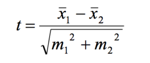
Ошибки репрезентативности были подробно объяснены мною в статье по доверительным интервалам. Поэтому я рекомендую вам ознакомиться с ней, чтобы лучше разобраться, что такое ошибки репрезентативности, что такое выборка, как она соотносится с генеральной совокупностью.
Для того, чтобы не тратить время, я в принципе все уже рассчитал по каждой из групп: средняя (x̅) ,стандартное отклонение (SD) и ошибка репрезентативности (mr).
Давайте остановимся на том, что же значат эти значения:
— средняя (x̅) это среднеарифметическое по 5 наблюдениям в каждой группе;
— если совсем упрощать значение стандартного отклонения (SD), то можно сказать, что оно представляет собой обобщенную среднюю отклонения каждого значения от среднего (стандартное отклонение показывает, насколько широко значения рассеяны (разбросаны) относительно средней). И дальше мы находим нечто среднее отклонений каждого варианта в группе от среднего;
— и ошибка репрезентативности она тоже находится достаточно просто: это как раз наше отклонение от средней некоторое стандартизованное, поэтому стандартное отклонение на размер выборки (mr=).
Итак, продолжаем. В ходе подстановки каждого значения в нашу формулу, мы находим, что t-критерий Стьюдента равен 3,78. Однако, я думаю, пока тем, кто не знаком со статистическими критериями, это мало о чем говорит.
Итак, теперь настает четвертый этап вопрос интерпретации. Ранее мы получили значение t-критерия в 3,78. Однако, что же это значит? Стоит отметить, что результаты статистических критериев и вообще их интерпретация не говорит о точном «да», либо «нет» в выводе, то есть рост отличается, либо рост не отличается. Всегда это вопрос определенной доли вероятности – доли вероятности ошибиться при констатации положительного результата (речь об ошибке первого рода (I type error, Alpha)). То есть, например, если мы скажем, что средний рост в начале ХХ и в начале XXI века отличаются с долей ошибкой меньше 5 %. Как раз эта величина в 5 % и фиксируется как достаточная для большинства биомедицинских исследований, помните, р больше, либо меньше 0,05.
Итак, как нам перейти от нашей t к р вероятности? Это сделать достаточно просто, стоит лишь воспользоваться табличными значениями t для определенных степеней свободы. Теперь вопрос: как найти эти степени свободы? Но это сделать достаточно просто. Для того, чтобы обнаружить степени свободы для наших групп, нужно лишь сложить количество наблюдений 5 и 5 в нашем случае и вычесть 2. В нашем случае степень свободы равна 8.
Итак, t=3,78, степень свободы равна 8. Переходим в табличное значение и получаем р вероятность – вероятность равна 0,005. То есть вероятность того, что мы ошибаемся при констатации факта различия роста ранее и сейчас, крайне мала – это 0,005 %, не 5 %, а 0,005 %. То есть мы можем говорить с высокой долей достоверности того, что наш рост сейчас в XXI веке и 100 лет назад отличаются.
Вот то, что касается расчета t-критерия Стьюдента и его интерпретации.
На этом наш разговор о t-критерии Стьюдента закончен. Спасибо, что ознакомились с этой статьей. Я очень надеюсь на вашу обратную связь. Пожалуйста, подписывайтесь на наш сайте, ставьте лайки, предлагайте свои темы для следующих выпусков. Спасибо большое за поддержку. С вами был Кирилл Мильчаков. Пока, до новых встреч!

Если Вам понравилась статья и оказалась полезной, Вы можете поделиться ею с коллегами и друзьями в социальных сетях:
Описательные статистики
Диалог Основные статистики и таблицы
Выводы
В ходе рассмотрения примера мы будем использовать вымышленные сведения, чтобы читатель мог провести необходимые преобразования самостоятельно.
Так, допустим, в ходе исследований изучали влияние препарата А на содержание вещества В (в ммоль/г) в ткани С и концентрацию вещества D в крови (в ммоль/л) у пациентов, разделенных по какому-то признаку Е на 3 группы равного объема (n = 10). Результаты такого выдуманного исследования приведены в таблице:
| Содержание вещества B, ммоль/г |
Вещество D, ммоль/л |
||||||
|---|---|---|---|---|---|---|---|
|
исходное содержание в крови |
прирост концентрации |
||||||
|
группа 1 |
группа 2 |
группа 3 |
группа 1 |
группа 2 |
группа 3 |
группа 2 |
группа 3 |
|
12 |
8 |
8 |
0,7 |
0,8 |
0,8 |
4 |
4 |
|
13 |
8 |
9 |
1,4 |
0,9 |
0,9 |
5 |
3 |
|
14 |
9 |
9 |
1,8 |
2,5 |
2,3 |
4 |
3,5 |
|
15 |
10 |
11 |
1,1 |
1,2 |
2,0 |
3,5 |
2 |
|
14 |
7 |
12 |
1,6 |
1,3 |
1,4 |
5 |
1 |
|
13 |
7 |
12 |
1,7 |
1,5 |
1,6 |
5 |
1,5 |
|
13 |
9 |
13 |
1,3 |
1,6 |
1,3 |
3,5 |
1 |
|
10 |
9 |
13 |
1,4 |
2,1 |
1,7 |
4 |
1,5 |
|
11 |
11 |
12 |
1,5 |
2,0 |
1,5 |
2 |
2 |
|
16 |
6 |
11 |
2,2 |
1,0 |
1,6 |
5 |
2 |
Хотим вас предупредить, что выборки объема 10 рассматриваются нами для простоты представления данных и вычислений, на практике такого объема выборок обычно оказывается недостаточно для формирования статистического заключения.
В качестве примера рассмотрим данные 1-го столбца таблицы.
Описательные статистики
Выборочное среднее
Среднее арифметическое, которое очень часто называют просто «среднее», получают путем сложения всех значений и деления этой суммы на число значений в наборе. Это можно показать с помощью алгебраической формулы. Набор n наблюдений переменной x можно изобразить как x1, x2, х3, …, xn
Формула для определения среднего арифметического наблюдений  (произносится «икс с чертой»):
= (Х1 + Х2 + … + Xn) / n
= (12 + 13 + 14 + 15 + 14 + 13 + 13 + 10 + 11 + 16) / 10 = 13,1;
Выборочная дисперсия
Один из способов измерения рассеяния данных заключается в том, чтобы определить степень отклонения каждого наблюдения от средней арифметической. Очевидно, что чем больше отклонение, тем больше изменчивость, вариабельность наблюдений. Однако мы не можем использовать среднее этих отклоненийкак меру рассеяния, потому что положительные отклонения компенсируют отрицательные отклонения (их сумма равна нулю). Чтобы решить эту проблему, мы возводим в квадрат каждое отклонение и находим среднее возведенных в квадрат отклонений; эта величина называется вариацией, или дисперсией. Возьмем n наблюдений x1, x2, х3, …, xn, средняя которых равняется  . Вычисляем дисперсию, обычно обозначаемую как s2, этих наблюдений:

Выборочная дисперсия данного показателя равна s2 = 3,2.
Среднеквадратичное отклонение
Стандартное (среднеквадратичное) отклонение — это положительный квадратный корень из дисперсии. На примере n наблюдений это выглядит следующим образом:

Мы можем представить себе стандартное отклонение как своего рода среднее отклонение наблюдений от среднего. Оно вычисляется в тех же единицах (размерностях), что и исходные данные.
s = sqrt (s2) = sqrt (3,2) = 1,79 [sqrt (x) — функция извлечения квадратного корня из х].
Коэффициент вариации
Если разделить стандартное отклонение на среднее арифметическое и выразить результат в процентах, то получится коэффициент вариации.
CV = (1,79 / 13,1) * 100% = 13,7
Ошибка выборочного среднего
1,79 / sqrt (10) = 0,57 [sqrt (x)- функция извлечения квадратного корня из х];
Коэффициент Стьюдента t (одновыборочный t-критерий)
Применяется для проверки гипотезы об отличии среднего значения  от некоторого известного значения m

Количество степеней свободы рассчитывается как f=n-1.
В данном случае доверительный интервал для среднего заключен между границами 11,87 и 14,39.
Для уровня доверительной вероятности 95% m=11,87 или m=14,39, то есть = |13,1-11,82| = |13,1-14,38| = 1,28
Соответственно, в данном случае для числа степеней свободы f = 10 — 1 = 9 и уровня доверительной вероятности 95% t=2,26.
Диалог Основные статистики и таблицы
В модуле Основные статистики и таблицы выберем Описательные статистики.

Откроется диалоговое окно Описательные статистики.
В поле Перменные выберем Группу 1.

Нажав на Ок, получим таблицы результатов с описательными статистиками выбранных переменных.

Чтобы посчитать t-критерий Стьюдента, в модуле Основные статистики и таблицы выберем Одновыборочный t-критерий.

Откроется диалоговое окно Одновыборочный t-критерий.

Предположим, нам известно, что среднее содержание вещества B в ткани С равно 11.

Таблица результатов с описательными статистиками и t-критерием Стьюдента выглядит следующим образом:

Нам пришлось отвергнуть гипотезу о том, что среднее содержание вещества В в ткани С равно 11.
Так как вычисленное значение критерия больше табличного (2,26), нулевая гипотеза отвергается на выбранном уровне значимости, и различия между выборкой и известной величиной признаются статистически значимыми. Таким образом, вывод о существовании различий, сделанный с помощью критерия Cтьюдента, подтверждается с помощью данного метода.
Выводы
Статистики и процедуры, включенные в одноименный модуль, условно называются основными статистиками и рассматриваются в одной группе, т.к. обычно они используются совместно, особенно на начальной, разведочной стадии анализа данных. Эти статистики являются базовыми и полезны для самых разнообразных исследований. Вычисление описательных статистик является неотъемлемой частью любого статистического анализа.
Связанные определения:
Выборочное среднее, среднее значение выборки
Выброс
Дисперсия (рассеяние, разброс)
Дисперсия выборки (выборочная дисперсия)
Коэффициент вариации
Максимум
Математическое ожидание дискретной случайной величины
Математическое ожидание непрерывной случайной величины
Медиана
Меры дисперсии, меры разброса
Минимум
Мода
Описательные статистики
Описательный анализ
Параметрические методы статистики
Параметры рассеяния
Параметры центральной тенденции
Среднее значение
Среднеквадратичное отклонение популяции
Стандартная ошибка среднего
Стандартное отклонение
В начало
Содержание портала
Проверка статистической гипотезы позволяет сделать строгий вывод о характеристиках генеральной совокупности на основе выборочных данных. Гипотезы бывают разные. Одна из них – это гипотеза о средней (математическом ожидании). Суть ее в том, чтобы на основе только имеющейся выборки сделать корректное заключение о том, где может или не может находится генеральная средняя (точную правду мы никогда не узнаем, но можем сузить круг поиска).
Распределение Стьюдента
Общий подход в проверке гипотез описан здесь, поэтому сразу к делу. Предположим для начала, что выборка извлечена из нормальной совокупности случайных величин X с генеральной средней μ и дисперсией σ2. Средняя арифметическая из этой выборки, очевидно, сама является случайной величиной. Если извлечь много таких выборок и посчитать по ним средние, то они также будут иметь нормальное распределение с математическим ожиданием μ и дисперсией

Тогда случайная величина

имеет стандартное нормальное распределение со всеми вытекающими отсюда последствиями. Например, с вероятностью 95% ее значение не выйдет за пределы ±1,96.
Однако такой подход будет корректным, если известна генеральная дисперсия. В реальности, как правило, она не известна. Вместо нее берут оценку – несмещенную выборочную дисперсию:

где
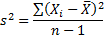
Возникает вопрос: будет ли генеральная средняя c вероятностью 95% находиться в пределах ±1,96sx̅. Другими словами, являются ли распределения случайных величин
и

эквивалентными.
Впервые этот вопрос был поставлен (и решен) одним химиком, который трудился на пивной фабрике Гиннесса в г. Дублин (Ирландия). Химика звали Уильям Сили Госсет и он брал пробы пива для проведения химического анализа. В какой-то момент, видимо, Уильяма стали терзать смутные сомнения на счет распределения средних. Оно получалось немного более размазанным, чем должно быть у нормального распределения.
Собрав математическое обоснование и рассчитав значения функции обнаруженного им распределения, химик из Дублина Уильям Госсет написал заметку, которая была опубликована в мартовском выпуске 1908 года журнала «Биометрика» (главред – Карл Пирсон). Гиннесс строго-настрого запретил выдавать секреты пивоварения, и Госсет подписался псевдонимом Стьюдент.
Несмотря на то что, К. Пирсон уже изобрел распределение Хи-квадрат, все-таки всеобщее представление о нормальности еще доминировало. Никто не собирался думать, что распределение выборочных оценок может быть не нормальным. Поэтому статья У. Госсета осталась практически не замеченной и забытой. И только Рональд Фишер по достоинству оценил открытие Госсета. Фишер использовал новое распределение в своих работах и дал ему название t-распределение Стьюдента. Критерий для проверки гипотез, соответственно, стал t-критерием Стьюдента. Так произошла «революция» в статистике, которая шагнула в эру анализа выборочных данных. Это был краткий экскурс в историю.
Посмотрим, что же мог увидеть У. Госсет. Сгенерируем 20 тысяч нормальных выборок из 6-ти наблюдений со средней (X̅) 50 и среднеквадратичным отклонением (σ) 10. Затем нормируем выборочные средние, используя генеральную дисперсию:
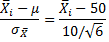
Получившиеся 20 тысяч средних сгруппируем в интервалы длинной 0,1 и подсчитаем частоты. Изобразим на диаграмме фактическое (Norm) и теоретическое (ENorm) распределение частот выборочных средних.
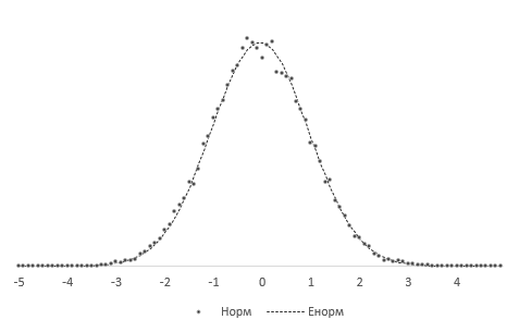
Точки (наблюдаемые частоты) практически совпадают с линией (теоретическими частотами). Оно и понятно, ведь данные взяты из одной и то же генеральной совокупности, а отличия – это лишь ошибки выборки.
Проведем новый эксперимент. Нормируем средние, используя выборочную дисперсию.
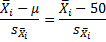
Снова подсчитаем частоты и нанесем их на диаграмму в виде точек, оставив для сравнения линию стандартного нормального распределения. Обозначим эмпирическое частоты средних, скажем, через букву t.
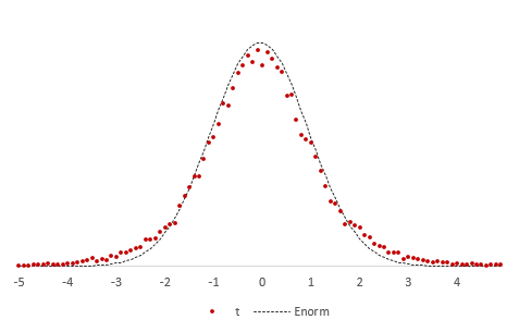
Видно, что распределения на этот раз не очень-то и совпадают. Близки, да, но не одинаковы. Хвосты стали более «тяжелыми».
У Госсета-Стьюдента не было последней версии MS Excel, но именно этот эффект он и заметил. Почему так получается? Объяснение заключается в том, что случайная величина
зависит не только от ошибки выборки (числителя), но и от стандартной ошибки средней (знаменателя), которая также является случайной величиной.
Давайте немного разберемся, какое распределение должно быть у такой случайной величины. Вначале придется кое-что вспомнить (или узнать) из математической статистики. Есть такая теорема Фишера, которая гласит, что в выборке из нормального распределения:
1. средняя X̅ и выборочная дисперсия s2 являются независимыми величинами;
2. соотношение выборочной и генеральной дисперсии, умноженное на количество степеней свободы, имеет распределение χ2(хи-квадрат) с таким же количеством степеней свободы, т.е.

где k – количество степеней свободы (на английском degrees of freedom (d.f.))
Вернемся к распределению средней. Разделим числитель и знаменатель выражения
на σX̅. Получим

Числитель – это стандартная нормальная случайная величина (обозначим ξ (кси)). Знаменатель выразим из теоремы Фишера.

Тогда исходное выражение примет вид

Это и есть t-критерий Стьюдента в общем виде (стьюдентово отношение). Вывести функцию его распределения можно уже непосредственно, т.к. распределения обеих случайных величин в данном выражении известны. Оставим это удовольствие математикам.
Функция t-распределения Стьюдента имеет довольно сложную для понимания формулу, поэтому не имеет смысла ее разбирать. Вероятности и квантили t-критерия приведены в специальных таблицах распределения Стьюдента и забиты в функции разных ПО вроде Excel.
Итак, вооружившись новыми знаниями, вы сможете понять официальное определение распределения Стьюдента.
Случайной величиной, подчиняющейся распределению Стьюдента с k степенями свободы, называется отношение независимых случайных величин
где ξ распределена по стандартному нормальному закону, а χ2k подчиняется распределению χ2 c k степенями свободы.
Таким образом, формула критерия Стьюдента для средней арифметической
есть частный случай стьюдентова отношения
Из формулы и определения следует, что распределение т-критерия Стьюдента зависит лишь от количества степеней свободы.
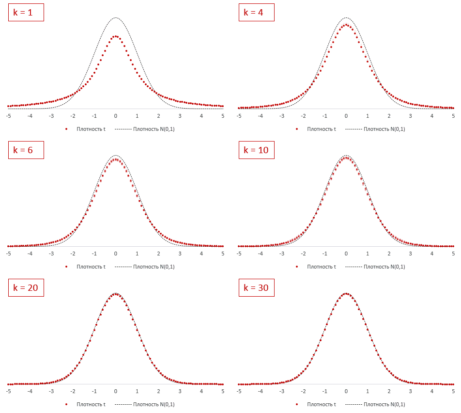
При k > 30 t-критерий практически не отличается от стандартного нормального распределения.
В отличие от хи-квадрат, t-критерий может быть одно- и двусторонним. Обычно пользуются двусторонним, предполагая, что отклонение может происходить в обе стороны от средней. Но если условие задачи допускает отклонение только в одну сторону, то разумно применять односторонний критерий. От этого немного увеличивается мощность критерия.
Несмотря на то, что открытие Стьюдента в свое время совершило переворот в статистике, t-критерий все же довольно сильно ограничен в возможностях применения, т.к. сам по себе происходит из предположения о нормальном распределении исходных данных. Если данные не являются нормальными (что обычно и бывает), то и t-критерий уже не будет иметь распределения Стьюдента. Однако в силу действия центральной предельной теоремы средняя даже у ненормальных данных быстро приобретает колоколообразную форму распределения.
Рассмотрим, для примера, данные, имеющие выраженный скос вправо, как у распределения хи-квадрат с 5-ю степенями свободы.
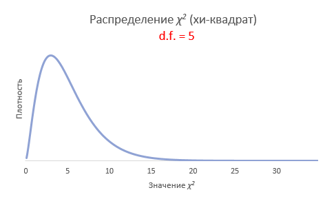
Теперь создадим 20 тысяч выборок и будет наблюдать, как меняется распределение средних в зависимости от их объема.
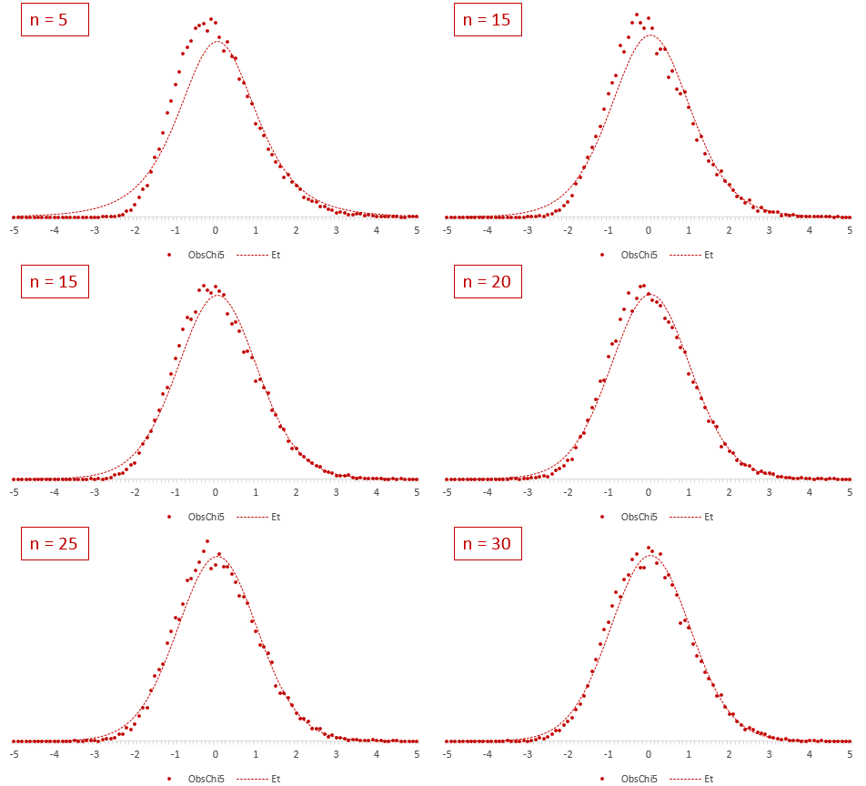
Отличие довольно заметно в малых выборках до 15-20-ти наблюдений. Но дальше оно стремительно исчезает. Таким образом, ненормальность распределения – это, конечно, нехорошо, но некритично.
Больше всего t-критерий «боится» выбросов, т.е. аномальных отклонений. Возьмем 20 тыс. нормальных выборок по 15 наблюдений и в часть из них добавим по одному случайном выбросу.
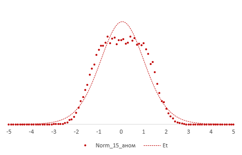
Картина получается нерадостная. Фактические частоты средних сильно отличаются от теоретических. Использование t-распределения в такой ситуации становится весьма рискованной затеей.
Итак, в не очень малых выборках (от 15-ти наблюдений) t-критерий относительно устойчив к ненормальному распределению исходных данных. А вот выбросы в данных сильно искажают распределение t-критерия, что, в свою очередь, может привести к ошибкам статистического вывода, поэтому от аномальных наблюдений следует избавиться. Часто из выборки удаляют все значения, выходящие за пределы ±2 стандартных отклонения от средней.
Пример проверки гипотезы о математическом ожидании с помощью t- критерия Стьюдента в MS Excel
В Excel есть несколько функций, связанных с t-распределением. Рассмотрим их.
СТЬЮДЕНТ.РАСП – «классическое» левостороннее t-распределение Стьюдента. На вход подается значение t-критерия, количество степеней свободы и опция (0 или 1), определяющая, что нужно рассчитать: плотность или значение функции. На выходе получаем, соответственно, плотность или вероятность того, что случайная величина окажется меньше указанного в аргументе t-критерия, т.е. левосторонний p-value.
СТЬЮДЕНТ.РАСП.2Х – двухсторонне распределение. В качестве аргумента подается абсолютное значение (по модулю) t-критерия и количество степеней свободы. На выходе получаем вероятность получить такое или еще больше значение t-критерия (по модулю), т.е. фактический уровень значимости (p-value).
СТЬЮДЕНТ.РАСП.ПХ – правостороннее t-распределение. Так, 1-СТЬЮДЕНТ.РАСП(2;5;1) = СТЬЮДЕНТ.РАСП.ПХ(2;5) = 0,05097. Если t-критерий положительный, то полученная вероятность – это p-value.
СТЬЮДЕНТ.ОБР – используется для расчета левостороннего обратного значения t-распределения. В качестве аргумента подается вероятность и количество степеней свободы. На выходе получаем соответствующее этой вероятности значение t-критерия. Отсчет вероятности идет слева. Поэтому для левого хвоста нужен сам уровень значимости α, а для правого 1 — α.
СТЬЮДЕНТ.ОБР.2Х – обратное значение для двухстороннего распределения Стьюдента, т.е. значение t-критерия (по модулю). Также на вход подается уровень значимости α. Только на этот раз отсчет ведется с двух сторон одновременно, поэтому вероятность распределяется на два хвоста. Так, СТЬЮДЕНТ.ОБР(1-0,025;5) = СТЬЮДЕНТ.ОБР.2Х(0,05;5) = 2,57058
СТЬЮДЕНТ.ТЕСТ – функция для проверки гипотезы о равенстве математических ожиданий в двух выборках. Заменяет кучу расчетов, т.к. достаточно указать лишь два диапазона с данными и еще пару параметров. На выходе получим p-value.
ДОВЕРИТ.СТЬЮДЕНТ – расчет доверительного интервала средней с учетом t-распределения.
Рассмотрим такой учебный пример. На предприятии фасуют цемент в мешки по 50кг. В силу случайности в отдельно взятом мешке допускается некоторое отклонение от ожидаемой массы, но генеральная средняя должна оставаться 50кг. В отделе контроля качества случайным образом взвесили 9 мешков и получили следующие результаты: средняя масса (X̅) составила 50,3кг, среднеквадратичное отклонение (s) – 0,5кг.
Согласуется ли полученный результат с нулевой гипотезой о том, что генеральная средняя равна 50кг? Другими словами, можно ли получить такой результат по чистой случайности, если оборудование работает исправно и выдает среднее наполнение 50 кг? Если гипотеза не будет отклонена, то полученное различие вписывается в диапазон случайных колебаний, если же гипотеза будет отклонена, то, скорее всего, в настройках аппарата, заполняющего мешки, произошел сбой. Требуется его проверка и настройка.
Краткое условие в обще принятых обозначениях выглядит так.
H0: μ = 50 кг
Ha: μ ≠ 50 кг
Есть основания предположить, что распределение заполняемости мешков подчиняются нормальному распределению (или не сильно от него отличается). Значит, для проверки гипотезы о математическом ожидании можно использовать t-критерий Стьюдента. Случайные отклонения могут происходить в любую сторону, значит нужен двусторонний t-критерий.
Вначале применим допотопные средства: ручной расчет t-критерия и сравнение его с критическим табличным значением. Расчетный t-критерий:
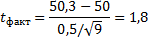
Теперь определим, выходит ли полученное число за критический уровень при уровне значимости α = 0,05. Воспользуемся таблицей для критерия Стьюдента (есть в любом учебнике по статистике).
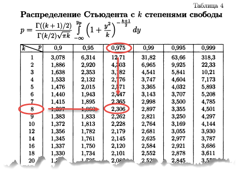
По столбцам идет вероятность правой части распределения, по строкам – число степеней свободы. Нас интересует двусторонний t-критерий с уровнем значимости 0,05, что равносильно t-значению для половины уровня значимости справа: 1 — 0,05/2 = 0,975. Количество степеней свободы – это объем выборки минус 1, т.е. 9 — 1 = 8. На пересечении находим табличное значение t-критерия – 2,306. Если бы мы использовали стандартное нормальное распределение, то критической точкой было бы значение 1,96, а тут она больше, т.к. t-распределение на небольших выборках имеет более приплюснутый вид.
Сравниваем фактическое (1,8) и табличное значение (2.306). Расчетный критерий оказался меньше табличного. Следовательно, имеющиеся данные не противоречат гипотезе H0 о том, что генеральная средняя равна 50 кг (но и не доказывают ее). Это все, что мы можем узнать, используя таблицы. Можно, конечно, еще p-value попробовать найти, но он будет приближенным. А, как правило, именно p-value используется для проверки гипотез. Поэтому далее переходим в Excel.
Готовой функции для расчета t-критерия в Excel нет. Но это и не страшно, ведь формула t-критерия Стьюдента довольно проста и ее можно легко соорудить прямо в ячейке Excel.
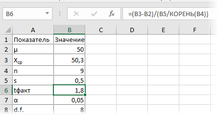
Получили те же 1,8. Найдем вначале критическое значение. Альфа берем 0,05, критерий двусторонний. Нужна функция обратного значения t-распределения для двухсторонней гипотезы СТЬЮДЕНТ.ОБР.2Х.
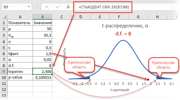
Полученное значение отсекает критическую область. Наблюдаемый t-критерий в нее не попадает, поэтому гипотеза не отклоняется.
Однако это тот же способ проверки гипотезы с помощью табличного значения. Более информативно будет рассчитать p-value, т.е. вероятность получить наблюдаемое или еще большее отклонение от средней 50кг, если эта гипотеза верна. Потребуется функция распределения Стьюдента для двухсторонней гипотезы СТЬЮДЕНТ.РАСП.2Х.
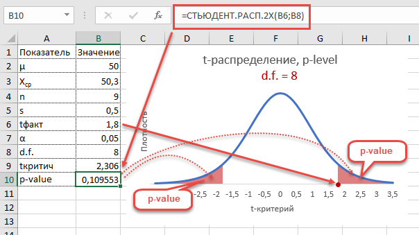
P-value равен 0,1096, что больше допустимого уровня значимости 0,05 – гипотезу не отклоняем. Но теперь можно судить о степени доказательства. P-value оказался довольно близок к тому уровню, когда гипотеза отклоняется, а это наводит на разные мысли. Например, что выборка оказалась слишком мала для обнаружения значимого отклонения.
Пусть через некоторое время отдел контроля снова решил проверить, как выдерживается стандарт заполняемости мешков. На этот раз для большей надежности было отобрано не 9, а 25 мешков. Интуитивно понятно, что разброс средней уменьшится, а, значит, и шансов найти сбой в системе становится больше.
Допустим, были получены те же значения средней и стандартного отклонения по выборке, что и в первый раз (50,3 и 0,5 соответственно). Рассчитаем t-критерий.
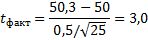
Критическое значение для 24-х степеней свободы и α = 0,05 составляет 2,064. На картинке ниже видно, что t-критерий попадает в область отклонения гипотезы.
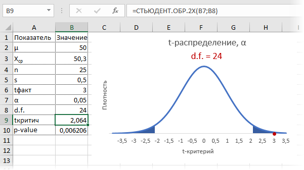
Можно сделать вывод о том, что с доверительной вероятностью более 95% генеральная средняя отличается от 50кг. Для большей убедительности посмотрим на p-value (последняя строка в таблице). Вероятность получить среднюю с таким или еще большим отклонением от 50, если гипотеза верна, составляет 0,0062, или 0,62%, что при однократном измерении практически невозможно. В общем, гипотезу отклоняем, как маловероятную.
Расчет доверительного интервала для математического ожидания с помощью t-распределения Стьюдента в Excel
С проверкой гипотез тесно связан еще один статистический метод – расчет доверительных интервалов. Если в полученный интервал попадает значение, соответствующее нулевой гипотезе, то это равносильно тому, что нулевая гипотеза не отклоняется. В противном случае, гипотеза отклоняется с соответствующей доверительной вероятностью. В некоторых случаях аналитики вообще не проверяют гипотез в классическом виде, а рассчитывают только доверительные интервалы. Такой подход позволяет извлечь еще больше полезной информации.
Рассчитаем доверительные интервалы для средней при 9 и 25 наблюдениях. Для этого воспользуемся функцией Excel ДОВЕРИТ.СТЬЮДЕНТ. Здесь, как ни странно, все довольно просто. В аргументах функции нужно указать только уровень значимости α, стандартное отклонение по выборке и размер выборки. На выходе получим полуширину доверительного интервала, то есть значение которое нужно отложить по обе стороны от средней. Проведя расчеты и нарисовав наглядную диаграмму, получим следующее.
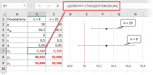
Как видно, при выборке в 9 наблюдений значение 50 попадает в доверительный интервал (гипотеза не отклоняется), а при 25-ти наблюдениях не попадает (гипотеза отклоняется). При этом в эксперименте с 25-ю мешками можно утверждать, что с вероятностью 97,5% генеральная средняя превышает 50,1 кг (нижняя граница доверительного интервала равна 50,094кг). А это довольно ценная информация.
Таким образом, мы решили одну и ту же задачу тремя способами:
1. Древним подходом, сравнивая расчетное и табличное значение t-критерия
2. Более современным, рассчитав p-value, добавив степень уверенности при отклонении гипотезы.
3. Еще более информативным, рассчитав доверительный интервал и получив минимальное значение генеральной средней.
Важно помнить, что t-критерий относится к параметрическим методам, т.к. основан на нормальном распределении (у него два параметра: среднее и дисперсия). Поэтому для его успешного применения важна хотя бы приблизительная нормальность исходных данных и отсутствие выбросов.
Напоследок предлагаю видеоролик о том, как рассчитать критерий Стьюдента и проверить гипотезу о генеральной средней в Excel.
Иногда просят объяснить, как делаются такие наглядные диаграммы с распределением. Ниже можно скачать файл, где проводились расчеты для этой статьи.
Скачать файл с примером.
Всего доброго, будьте здоровы.
Поделиться в социальных сетях: