
17 авг. 2022 г.
читать 1 мин
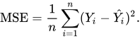
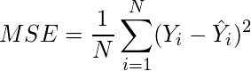
Среднеквадратическая ошибка (MSE) — это распространенный способ измерения точности предсказания модели. Он рассчитывается как:
MSE = (1/n) * Σ(фактическое – прогноз) 2
куда:
- Σ — причудливый символ, означающий «сумма».
- n – размер выборки
- фактический – фактическое значение данных
- прогноз – прогнозируемое значение данных
Чем ниже значение MSE, тем лучше модель способна точно предсказывать значения.
Как рассчитать MSE в Python
Мы можем создать простую функцию для вычисления MSE в Python:
import numpy as np

def mse(actual, pred):
 actual, pred = np.array(actual), np.array(pred)
 return np.square(np.subtract(actual,pred)).mean()
Затем мы можем использовать эту функцию для вычисления MSE для двух массивов: одного, содержащего фактические значения данных, и другого, содержащего прогнозируемые значения данных.
actual = [12, 13, 14, 15, 15, 22, 27]
pred = [11, 13, 14, 14, 15, 16, 18]

mse(actual, pred)

17.0
Среднеквадратическая ошибка (MSE) для этой модели оказывается равной 17,0 .
На практике среднеквадратическая ошибка (RMSE) чаще используется для оценки точности модели. Как следует из названия, это просто квадратный корень из среднеквадратичной ошибки.
Мы можем определить аналогичную функцию для вычисления RMSE:
import numpy as np

def rmse(actual, pred):
 actual, pred = np.array(actual), np.array(pred)
 return np.sqrt(np.square(np.subtract(actual,pred)).mean())
Затем мы можем использовать эту функцию для вычисления RMSE для двух массивов: одного, содержащего фактические значения данных, и другого, содержащего прогнозируемые значения данных.
actual = [12, 13, 14, 15, 15, 22, 27]
pred = [11, 13, 14, 14, 15, 16, 18]

rmse(actual, pred)

4.1231
Среднеквадратическая ошибка (RMSE) для этой модели оказывается равной 4,1231 .
Дополнительные ресурсы
Калькулятор среднеквадратичной ошибки (MSE)
Как рассчитать среднеквадратичную ошибку (MSE) в Excel
The mean squared error is a common way to measure the prediction accuracy of a model. In this tutorial, you’ll learn how to calculate the mean squared error in Python. You’ll start off by learning what the mean squared error represents. Then you’ll learn how to do this using Scikit-Learn (sklean), Numpy, as well as from scratch.
What is the Mean Squared Error
The mean squared error measures the average of the squares of the errors. What this means, is that it returns the average of the sums of the square of each difference between the estimated value and the true value.
The MSE is always positive, though it can be 0 if the predictions are completely accurate. It incorporates the variance of the estimator (how widely spread the estimates are) and its bias (how different the estimated values are from their true values).
The formula looks like below:
Now that you have an understanding of how to calculate the MSE, let’s take a look at how it can be calculated using Python.
Interpreting the Mean Squared Error
The mean squared error is always 0 or positive. When a MSE is larger, this is an indication that the linear regression model doesn’t accurately predict the model.
An important piece to note is that the MSE is sensitive to outliers. This is because it calculates the average of every data point’s error. Because of this, a larger error on outliers will amplify the MSE.
There is no “target” value for the MSE. The MSE can, however, be a good indicator of how well a model fits your data. It can also give you an indicator of choosing one model over another.
Loading a Sample Pandas DataFrame
Let’s start off by loading a sample Pandas DataFrame. If you want to follow along with this tutorial line-by-line, simply copy the code below and paste it into your favorite code editor.
# Importing a sample Pandas DataFrame
import pandas as pd

df = pd.DataFrame.from_dict({
    'x': [1,2,3,4,5,6,7,8,9,10],
    'y': [1,2,2,4,4,5,6,7,9,10]})

print(df.head())
#    x  y
# 0  1  1
# 1  2  2
# 2  3  2
# 3  4  4
# 4  5  4
You can see that the editor has loaded a DataFrame containing values for variables x and y. We can plot this data out, including the line of best fit using Seaborn’s .regplot() function:
# Plotting a line of best fit
import seaborn as sns
import matplotlib.pyplot as plt
sns.regplot(data=df, x='x', y='y', ci=None)
plt.ylim(bottom=0)
plt.xlim(left=0)
plt.show()
This returns the following visualization:
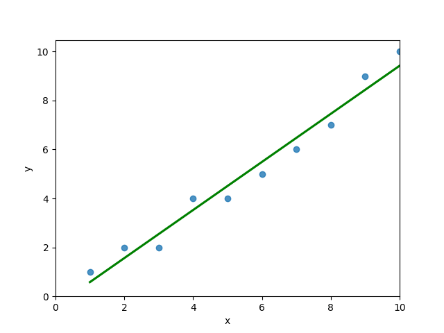
The mean squared error calculates the average of the sum of the squared differences between a data point and the line of best fit. By virtue of this, the lower a mean sqared error, the more better the line represents the relationship.
We can calculate this line of best using Scikit-Learn. You can learn about this in this in-depth tutorial on linear regression in sklearn. The code below predicts values for each x value using the linear model:
# Calculating prediction y values in sklearn
from sklearn.linear_model import LinearRegression

model = LinearRegression()
model.fit(df[['x']], df['y'])
y_2 = model.predict(df[['x']])
df['y_predicted'] = y_2
print(df.head())

# Returns:
#    x  y  y_predicted
# 0  1  1     0.581818
# 1  2  2     1.563636
# 2  3  2     2.545455
# 3  4  4     3.527273
# 4  5  4     4.509091
Calculating the Mean Squared Error with Scikit-Learn
The simplest way to calculate a mean squared error is to use Scikit-Learn (sklearn). The metrics module comes with a function, mean_squared_error() which allows you to pass in true and predicted values.
Let’s see how to calculate the MSE with sklearn:
# Calculating the MSE with sklearn
from sklearn.metrics import mean_squared_error
mse = mean_squared_error(df['y'], df['y_predicted'])
print(mse)

# Returns: 0.24727272727272714
This approach works very well when you’re already importing Scikit-Learn. That said, the function works easily on a Pandas DataFrame, as shown above.
In the next section, you’ll learn how to calculate the MSE with Numpy using a custom function.
Calculating the Mean Squared Error from Scratch using Numpy
Numpy itself doesn’t come with a function to calculate the mean squared error, but you can easily define a custom function to do this. We can make use of the subtract() function to subtract arrays element-wise.
# Definiting a custom function to calculate the MSE
import numpy as np

def mse(actual, predicted):
    actual = np.array(actual)
    predicted = np.array(predicted)
    differences = np.subtract(actual, predicted)
    squared_differences = np.square(differences)
    return squared_differences.mean()

print(mse(df['y'], df['y_predicted']))

# Returns: 0.24727272727272714
The code above is a bit verbose, but it shows how the function operates. We can cut down the code significantly, as shown below:
# A shorter version of the code above
import numpy as np

def mse(actual, predicted):
    return np.square(np.subtract(np.array(actual), np.array(predicted))).mean()

print(mse(df['y'], df['y_predicted']))

# Returns: 0.24727272727272714
Conclusion
In this tutorial, you learned what the mean squared error is and how it can be calculated using Python. First, you learned how to use Scikit-Learn’s mean_squared_error() function and then you built a custom function using Numpy.
The MSE is an important metric to use in evaluating the performance of your machine learning models. While Scikit-Learn abstracts the way in which the metric is calculated, understanding how it can be implemented from scratch can be a helpful tool.
Additional Resources
To learn more about related topics, check out the tutorials below:
- Pandas Variance: Calculating Variance of a Pandas Dataframe Column
- Calculate the Pearson Correlation Coefficient in Python
- How to Calculate a Z-Score in Python (4 Ways)
- Official Documentation from Scikit-Learn
Improve Article
Save Article
Improve Article
Save Article
The Mean Squared Error (MSE) or Mean Squared Deviation (MSD) of an estimator measures the average of error squares i.e. the average squared difference between the estimated values and true value. It is a risk function, corresponding to the expected value of the squared error loss. It is always non – negative and values close to zero are better. The MSE is the second moment of the error (about the origin) and thus incorporates both the variance of the estimator and its bias.
Steps to find the MSE
- Find the equation for the regression line.
(1)

- Insert X values in the equation found in step 1 in order to get the respective Y values i.e.
(2)

- Now subtract the new Y values (i.e.
 ) from the original Y values. Thus, found values are the error terms. It is also known as the vertical distance of the given point from the regression line.
(3)

- Square the errors found in step 3.
(4)
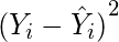
- Sum up all the squares.
(5)
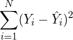
- Divide the value found in step 5 by the total number of observations.
(6)
Example:
Consider the given data points: (1,1), (2,1), (3,2), (4,2), (5,4)
You can use this online calculator to find the regression equation / line.
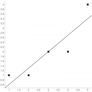
Regression line equation: Y = 0.7X – 0.1
| X | Y | |
|---|---|---|
| 1 | 1 | 0.6 |
| 2 | 1 | 1.29 |
| 3 | 2 | 1.99 |
| 4 | 2 | 2.69 |
| 5 | 4 | 3.4 |
Now, using formula found for MSE in step 6 above, we can get MSE = 0.21606
MSE using scikit – learn:
from sklearn.metrics import mean_squared_error
Y_true = [1,1,2,2,4]
Y_pred = [0.6,1.29,1.99,2.69,3.4]
mean_squared_error(Y_true,Y_pred)
Output: 0.21606
MSE using Numpy module:
import numpy as np
Y_true = [1,1,2,2,4]
Y_pred = [0.6,1.29,1.99,2.69,3.4]
MSE = np.square(np.subtract(Y_true,Y_pred)).mean()
Output: 0.21606
29.12.2019Python, Программы Python, Продвинутые компьютерные предметы
Среднее квадратичное отклонение (MSE) или Среднее квадратичное отклонение (MSD) оценщика измеряет среднее квадратов ошибок, то есть среднее квадратическое различие между оценочными значениями и истинным значением. Это функция риска, соответствующая ожидаемому значению квадрата потери ошибок. Это всегда неотрицательно, и значения, близкие к нулю, лучше. MSE является вторым моментом ошибки (относительно источника) и, таким образом, включает в себя как дисперсию оценки, так и ее смещение.
Шаги, чтобы найти MSE
- Найти уравнение для линии регрессии.
(1)

- Вставьте значения X в уравнение, найденное на шаге 1, чтобы получить соответствующие значения Y, т.е.
(2)

- Теперь вычтите новые значения Y (т.е.
 ) из исходных значений Y. Таким образом, найденные значения являются ошибочными терминами. Это также известно как вертикальное расстояние данной точки от линии регрессии.
(3)

- Возведите в квадрат ошибки, найденные в шаге 3.
(4)

- Подведите итог всех квадратов.
(5)

- Разделите значение, найденное на шаге 5, на общее количество наблюдений.
(6)

Пример:
Рассмотрим данные точки: (1,1), (2,1), (3,2), (4,2), (5,4)
Вы можете использовать этот онлайн калькулятор, чтобы найти уравнение / линию регрессии.

Уравнение линии регрессии: Y = 0,7X — 0,1
| X | Y | |
|---|---|---|
| 1 | 1 | 0.6 |
| 2 | 1 | 1.29 |
| 3 | 2 | 1.99 |
| 4 | 2 | 2.69 |
| 5 | 4 | 3.4 |
Теперь, используя формулу, найденную для MSE на шаге 6 выше, мы можем получить MSE = 0.21606
MSE, используя scikit — учиться:
from sklearn.metrics import mean_squared_error
Y_true = [1,1,2,2,4]
Y_pred = [0.6,1.29,1.99,2.69,3.4]
mean_squared_error(Y_true,Y_pred)
Output: 0.21606
MSE с использованием модуля Numpy:
import numpy as np
Y_true = [1,1,2,2,4]
Y_pred = [0.6,1.29,1.99,2.69,3.4]
MSE = np.square(np.subtract(Y_true,Y_pred)).mean()
Output: 0.21606
Рекомендуемые посты:
- ML | Потеря журнала и средняя квадратическая ошибка
- ML | Математическое объяснение СКО и R-квадрата ошибки
- Ошибка NZEC в Python
- Python | Ошибка подтверждения
- Ошибка с плавающей точкой в Python
- Python | 404 Обработка ошибок во Flask
- Python | Запрос пароля во время выполнения и завершение с сообщением об ошибке
- Python | Индекс ненулевых элементов в списке Python
- Python | Конвертировать список в массив Python
- Важные различия между Python 2.x и Python 3.x с примерами
- Чтение файловоподобных объектов Python из C | питон
- Python | Объединить значения ключа Python в список
- Python | Сортировать словари Python по ключу или значению
- Python | Набор 4 (словарь, ключевые слова в Python)
- Python | Добавить запись в библиотеки Python
Python | Средняя квадратическая ошибка
0.00 (0%) 0 votes
- sklearn.metrics.mean_squared_error(y_true, y_pred, *, sample_weight=None, multioutput=‘uniform_average’, squared=True)[source]
-
Mean squared error regression loss.
Read more in the User Guide.
- Parameters:
-
- y_truearray-like of shape (n_samples,) or (n_samples, n_outputs)
-
Ground truth (correct) target values.
- y_predarray-like of shape (n_samples,) or (n_samples, n_outputs)
-
Estimated target values.
- sample_weightarray-like of shape (n_samples,), default=None
-
Sample weights.
- multioutput{‘raw_values’, ‘uniform_average’} or array-like of shape (n_outputs,), default=’uniform_average’
-
Defines aggregating of multiple output values.
Array-like value defines weights used to average errors.- ‘raw_values’ :
-
Returns a full set of errors in case of multioutput input.
- ‘uniform_average’ :
-
Errors of all outputs are averaged with uniform weight.
- squaredbool, default=True
-
If True returns MSE value, if False returns RMSE value.
- Returns:
-
- lossfloat or ndarray of floats
-
A non-negative floating point value (the best value is 0.0), or an
array of floating point values, one for each individual target.
Examples
>>> from sklearn.metrics import mean_squared_error
>>> y_true = [3, -0.5, 2, 7]
>>> y_pred = [2.5, 0.0, 2, 8]
>>> mean_squared_error(y_true, y_pred)
0.375
>>> y_true = [3, -0.5, 2, 7]
>>> y_pred = [2.5, 0.0, 2, 8]
>>> mean_squared_error(y_true, y_pred, squared=False)
0.612...
>>> y_true = [[0.5, 1],[-1, 1],[7, -6]]
>>> y_pred = [[0, 2],[-1, 2],[8, -5]]
>>> mean_squared_error(y_true, y_pred)
0.708...
>>> mean_squared_error(y_true, y_pred, squared=False)
0.822...
>>> mean_squared_error(y_true, y_pred, multioutput='raw_values')
array([0.41666667, 1.        ])
>>> mean_squared_error(y_true, y_pred, multioutput=[0.3, 0.7])
0.825...
Examples using sklearn.metrics.mean_squared_error
Improve Article
Save Article
Improve Article
Save Article
In this article, we discussed the implementation of weighted mean square error using python.
Mean squared error is a vital statistical concept, that is nowadays widely used in Machine learning and Deep learning algorithm. Mean squared error is basically a measure of the average squared difference between the estimated values and the actual value. It is also called a mean squared deviation and is most of the time used to calibrate the accuracy of the predicted output. In this article, let us discuss a variety of mean squared errors called weighted mean square errors.
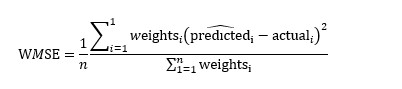
Weighted mean square error enables to provide more importance or additional weightage for a particular set of points (points of interest) when compared to others. When handling imbalanced data, a weighted mean square error can be a vital performance metric. Python provides a wide variety of packages to implement mean squared and weighted mean square at one go, here we can make use of simple functions to implement weighted mean squared error.
Formula to calculate the weighted mean square error:
Implementation of Weighted Mean Square Error
- For demonstration purposes let us create a sample data frame, with augmented actual and predicted values, as shown.
- Calculate the squared difference between actual and predicted values.
- Define the weights for each data point based on the importance
- Now, use the weights to calculate the weighted mean square error as shown
Code Implementation:
Python3
import pandas as pd
import numpy as np
import random
d = {'Actual': np.arange(0, 20, 2)*np.sin(2),
'Predicted': np.arange(0, 20, 2)*np.cos(2)}
data = pd.DataFrame(data=d)
y_weights = np.arange(2, 4, 0.2)
diff = (data['Actual']-data['Predicted'])**2
weighted_mean_sq_error = np.sum(diff * y_weights) / np.sum(y_weights)
Output:

Weighted Mean Square Error
Let us cross verify the result with the result of the scikit-learn package. to verify the correctness,
Code:
Python3
weighted_mean_sq_error_sklearn = np.average(
(data['Actual']-data['Predicted'])**2, axis=0, weights=y_weights)
weighted_mean_sq_error_sklearn
Output:

verify the result
Improve Article
Save Article
Improve Article
Save Article
In this article, we discussed the implementation of weighted mean square error using python.
Mean squared error is a vital statistical concept, that is nowadays widely used in Machine learning and Deep learning algorithm. Mean squared error is basically a measure of the average squared difference between the estimated values and the actual value. It is also called a mean squared deviation and is most of the time used to calibrate the accuracy of the predicted output. In this article, let us discuss a variety of mean squared errors called weighted mean square errors.
Weighted mean square error enables to provide more importance or additional weightage for a particular set of points (points of interest) when compared to others. When handling imbalanced data, a weighted mean square error can be a vital performance metric. Python provides a wide variety of packages to implement mean squared and weighted mean square at one go, here we can make use of simple functions to implement weighted mean squared error.
Formula to calculate the weighted mean square error:
Implementation of Weighted Mean Square Error
- For demonstration purposes let us create a sample data frame, with augmented actual and predicted values, as shown.
- Calculate the squared difference between actual and predicted values.
- Define the weights for each data point based on the importance
- Now, use the weights to calculate the weighted mean square error as shown
Code Implementation:
Python3
import pandas as pd
import numpy as np
import random
d = {'Actual': np.arange(0, 20, 2)*np.sin(2),
'Predicted': np.arange(0, 20, 2)*np.cos(2)}
data = pd.DataFrame(data=d)
y_weights = np.arange(2, 4, 0.2)
diff = (data['Actual']-data['Predicted'])**2
weighted_mean_sq_error = np.sum(diff * y_weights) / np.sum(y_weights)
Output:
Weighted Mean Square Error
Let us cross verify the result with the result of the scikit-learn package. to verify the correctness,
Code:
Python3
weighted_mean_sq_error_sklearn = np.average(
(data['Actual']-data['Predicted'])**2, axis=0, weights=y_weights)
weighted_mean_sq_error_sklearn
Output:
verify the result
Перевод
Ссылка на автора
Показатели эффективности прогнозирования по временным рядам дают сводку об умениях и возможностях модели прогноза, которая сделала прогнозы.
Есть много разных показателей производительности на выбор. Может быть непонятно, какую меру использовать и как интерпретировать результаты.
В этом руководстве вы узнаете показатели производительности для оценки прогнозов временных рядов с помощью Python.
Временные ряды, как правило, фокусируются на прогнозировании реальных значений, называемых проблемами регрессии. Поэтому показатели эффективности в этом руководстве будут сосредоточены на методах оценки реальных прогнозов.
После завершения этого урока вы узнаете:
- Основные показатели выполнения прогноза, включая остаточную ошибку прогноза и смещение прогноза.
- Вычисления ошибок прогноза временного ряда, которые имеют те же единицы, что и ожидаемые результаты, такие как средняя абсолютная ошибка.
- Широко используются вычисления ошибок, которые наказывают большие ошибки, такие как среднеквадратическая ошибка и среднеквадратичная ошибка.
Давайте начнем.

Ошибка прогноза (или остаточная ошибка прогноза)
ошибка прогноза рассчитывается как ожидаемое значение минус прогнозируемое значение.
Это называется остаточной ошибкой прогноза.
forecast_error = expected_value - predicted_valueОшибка прогноза может быть рассчитана для каждого прогноза, предоставляя временной ряд ошибок прогноза.
В приведенном ниже примере показано, как можно рассчитать ошибку прогноза для серии из 5 прогнозов по сравнению с 5 ожидаемыми значениями. Пример был придуман для демонстрационных целей.
expected = [0.0, 0.5, 0.0, 0.5, 0.0]
predictions = [0.2, 0.4, 0.1, 0.6, 0.2]
forecast_errors = [expected[i]-predictions[i] for i in range(len(expected))]
print('Forecast Errors: %s' % forecast_errors)
При выполнении примера вычисляется ошибка прогноза для каждого из 5 прогнозов. Список ошибок прогноза затем печатается.
Forecast Errors: [-0.2, 0.09999999999999998, -0.1, -0.09999999999999998, -0.2]Единицы ошибки прогноза совпадают с единицами прогноза. Ошибка прогноза, равная нулю, означает отсутствие ошибки или совершенный навык для этого прогноза.
Средняя ошибка прогноза (или ошибка прогноза)
Средняя ошибка прогноза рассчитывается как среднее значение ошибки прогноза.
mean_forecast_error = mean(forecast_error)Ошибки прогноза могут быть положительными и отрицательными. Это означает, что при вычислении среднего из этих значений идеальная средняя ошибка прогноза будет равна нулю.
Среднее значение ошибки прогноза, отличное от нуля, указывает на склонность модели к превышению прогноза (положительная ошибка) или занижению прогноза (отрицательная ошибка). Таким образом, средняя ошибка прогноза также называется прогноз смещения,
Ошибка прогноза может быть рассчитана непосредственно как среднее значение прогноза. В приведенном ниже примере показано, как среднее значение ошибок прогноза может быть рассчитано вручную.
expected = [0.0, 0.5, 0.0, 0.5, 0.0]
predictions = [0.2, 0.4, 0.1, 0.6, 0.2]
forecast_errors = [expected[i]-predictions[i] for i in range(len(expected))]
bias = sum(forecast_errors) * 1.0/len(expected)
print('Bias: %f' % bias)
При выполнении примера выводится средняя ошибка прогноза, также известная как смещение прогноза.
Bias: -0.100000Единицы смещения прогноза совпадают с единицами прогнозов. Прогнозируемое смещение нуля или очень маленькое число около нуля показывает несмещенную модель.
Средняя абсолютная ошибка
средняя абсолютная ошибка или MAE, рассчитывается как среднее значение ошибок прогноза, где все значения прогноза вынуждены быть положительными.
Заставить ценности быть положительными называется сделать их абсолютными. Это обозначено абсолютной функциейабс ()или математически показано как два символа канала вокруг значения:| Значение |,
mean_absolute_error = mean( abs(forecast_error) )кудаабс ()делает ценности позитивными,forecast_errorодна или последовательность ошибок прогноза, иимею в виду()рассчитывает среднее значение.
Мы можем использовать mean_absolute_error () функция из библиотеки scikit-learn для вычисления средней абсолютной ошибки для списка прогнозов. Пример ниже демонстрирует эту функцию.
from sklearn.metrics import mean_absolute_error
expected = [0.0, 0.5, 0.0, 0.5, 0.0]
predictions = [0.2, 0.4, 0.1, 0.6, 0.2]
mae = mean_absolute_error(expected, predictions)
print('MAE: %f' % mae)
При выполнении примера вычисляется и выводится средняя абсолютная ошибка для списка из 5 ожидаемых и прогнозируемых значений.
MAE: 0.140000Эти значения ошибок приведены в исходных единицах прогнозируемых значений. Средняя абсолютная ошибка, равная нулю, означает отсутствие ошибки.
Средняя квадратическая ошибка
средняя квадратическая ошибка или MSE, рассчитывается как среднее значение квадратов ошибок прогноза. Возведение в квадрат значений ошибки прогноза заставляет их быть положительными; это также приводит к большему количеству ошибок.
Квадратные ошибки прогноза с очень большими или выбросами возводятся в квадрат, что, в свою очередь, приводит к вытягиванию среднего значения квадратов ошибок прогноза, что приводит к увеличению среднего квадрата ошибки. По сути, оценка дает худшую производительность тем моделям, которые делают большие неверные прогнозы.
mean_squared_error = mean(forecast_error^2)Мы можем использовать mean_squared_error () функция из scikit-learn для вычисления среднеквадратичной ошибки для списка прогнозов. Пример ниже демонстрирует эту функцию.
from sklearn.metrics import mean_squared_error
expected = [0.0, 0.5, 0.0, 0.5, 0.0]
predictions = [0.2, 0.4, 0.1, 0.6, 0.2]
mse = mean_squared_error(expected, predictions)
print('MSE: %f' % mse)
При выполнении примера вычисляется и выводится среднеквадратическая ошибка для списка ожидаемых и прогнозируемых значений.
MSE: 0.022000Значения ошибок приведены в квадратах от предсказанных значений. Среднеквадратичная ошибка, равная нулю, указывает на совершенное умение или на отсутствие ошибки.
Среднеквадратическая ошибка
Средняя квадратичная ошибка, описанная выше, выражается в квадратах единиц прогнозов.
Его можно преобразовать обратно в исходные единицы прогнозов, взяв квадратный корень из среднего квадрата ошибки Это называется среднеквадратичная ошибка или RMSE.
rmse = sqrt(mean_squared_error)Это можно рассчитать с помощьюSQRT ()математическая функция среднего квадрата ошибки, рассчитанная с использованиемmean_squared_error ()функция scikit-learn.
from sklearn.metrics import mean_squared_error
from math import sqrt
expected = [0.0, 0.5, 0.0, 0.5, 0.0]
predictions = [0.2, 0.4, 0.1, 0.6, 0.2]
mse = mean_squared_error(expected, predictions)
rmse = sqrt(mse)
print('RMSE: %f' % rmse)
При выполнении примера вычисляется среднеквадратичная ошибка.
RMSE: 0.148324Значения ошибок RMES приведены в тех же единицах, что и прогнозы. Как и в случае среднеквадратичной ошибки, среднеквадратическое отклонение, равное нулю, означает отсутствие ошибки.
Дальнейшее чтение
Ниже приведены некоторые ссылки для дальнейшего изучения показателей ошибки прогноза временных рядов.
- Раздел 3.3 Измерение прогнозирующей точности, Практическое прогнозирование временных рядов с помощью R: практическое руководство,
- Раздел 2.5 Оценка точности прогноза, Прогнозирование: принципы и практика
- scikit-Learn Metrics API
- Раздел 3.3.4. Метрики регрессии, scikit-learn API Guide
Резюме
В этом руководстве вы обнаружили набор из 5 стандартных показателей производительности временных рядов в Python.
В частности, вы узнали:
- Как рассчитать остаточную ошибку прогноза и как оценить смещение в списке прогнозов.
- Как рассчитать среднюю абсолютную ошибку прогноза, чтобы описать ошибку в тех же единицах, что и прогнозы.
- Как рассчитать широко используемые среднеквадратические ошибки и среднеквадратичные ошибки для прогнозов.
Есть ли у вас какие-либо вопросы о показателях эффективности прогнозирования временных рядов или об этом руководстве?
Задайте свои вопросы в комментариях ниже, и я сделаю все возможное, чтобы ответить.
In this article, we are going to learn how to calculate the mean squared error in python? We are using two python libraries to calculate the mean squared error. NumPy and sklearn are the libraries we are going to use here. Also, we will learn how to calculate without using any module.
MSE is also useful for regression problems that are normally distributed. It is the mean squared error. So the squared error between the predicted values and the actual values. The summation of all the data points of the square difference between the predicted and actual values is divided by the no. of data points.
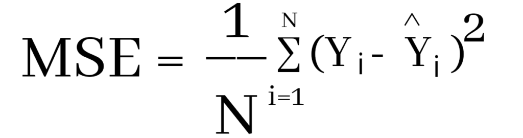
Where Yi and Ŷi represent the actual values and the predicted values, the difference between them is squared.
Derivation of Mean Squared Error
First to find the regression line for the values (1,3), (2,2), (3,6), (4,1), (5,5). The regression value for the value is y=1.6+0.4x. Next to find the new Y values. The new values for y are tabulated below.
| Given x value | Calculating y value | New y value |
|---|---|---|
| 1 | 1.6+0.4(1) | 2 |
| 2 | 1.6+0.4(2) | 2.4 |
| 3 | 1.6+0.4(3) | 2.8 |
| 4 | 1.6+0.4(4) | 3.2 |
| 5 | 1.6+0.4(5) | 3.6 |
Now to find the error ( Yi – Ŷi )
We have to square all the errors
By adding all the errors we will get the MSE
Line regression graph
Let us consider the values (1,3), (2,2), (3,6), (4,1), (5,5) to plot the graph.
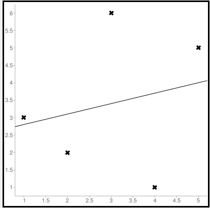
The straight line represents the predicted value in this graph, and the points represent the actual data. The difference between this line and the points is squared, known as mean squared error.
Also, Read | How to Calculate Square Root in Python
To get the Mean Squared Error in Python using NumPy
import numpy as np
true_value_of_y= [3,2,6,1,5]
predicted_value_of_y= [2.0,2.4,2.8,3.2,3.6]
MSE = np.square(np.subtract(true_value_of_y,predicted_value_of_y)).mean()
print(MSE)
Importing numpy library as np. Creating two variables. true_value_of_y holds an original value. predicted_value_of_y holds a calculated value. Next, giving the formula to calculate the mean squared error.
Output
3.6400000000000006
To get the MSE using sklearn
sklearn is a library that is used for many mathematical calculations in python. Here we are going to use this library to calculate the MSE
Syntax
sklearn.metrices.mean_squared_error(y_true, y_pred, *, sample_weight=None, multioutput='uniform_average', squared=True)
Parameters
- y_true – true value of y
- y_pred – predicted value of y
- sample_weight
- multioutput
- raw_values
- uniform_average
- squared
Returns
Mean squared error.
Code
from sklearn.metrics import mean_squared_error
true_value_of_y= [3,2,6,1,5]
predicted_value_of_y= [2.0,2.4,2.8,3.2,3.6]
mean_squared_error(true_value_of_y,predicted_value_of_y)
print(mean_squared_error(true_value_of_y,predicted_value_of_y))
From sklearn.metrices library importing mean_squared_error. Creating two variables. true_value_of_y holds an original value. predicted_value_of_y holds a calculated value. Next, giving the formula to calculate the mean squared error.
Output
3.6400000000000006
Calculating Mean Squared Error Without Using any Modules
true_value_of_y = [3,2,6,1,5]
predicted_value_of_y = [2.0,2.4,2.8,3.2,3.6]
summation_of_value = 0
n = len(true_value_of_y)
for i in range (0,n):
  difference_of_value = true_value_of_y[i] - predicted_value_of_y[i]
  squared_difference = difference_of_value**2
  summation_of_value = summation_of_value + squared_difference
MSE = summation_of_value/n
print ("The Mean Squared Error is: " , MSE)
Declaring the true values and the predicted values to two different variables. Initializing the variable summation_of_value is zero to store the values. len() function is useful to check the number of values in true_value_of_y. Creating for loop to iterate. Calculating the difference between true_value and the predicted_value. Next getting the square of the difference. Adding all the squared differences, we will get the MSE.
Output
The Mean Squared Error is: 3.6400000000000006
Calculate Mean Squared Error Using Negative Values
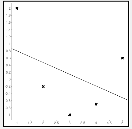
Now let us consider some negative values to calculate MSE. The values are (1,2), (3,-1), (5,0.6), (4,-0.7), (2,-0.2). The regression line equation is y=1.13-0.33x
The line regression graph for this value is:
New y values for this will be:
| Given x value | Calculating y value | New y value |
|---|---|---|
| 1 | 1.13-033(1) | 0.9 |
| 3 | 1.13-033(3) | 0.1 |
| 5 | 1.13-033(5) | -0.4 |
| 4 | 1.13-033(4) | -0.1 |
| 2 | 1.13-033(2) | 0.6 |
Code
>>> from sklearn.metrics import mean_squared_error
>>> y_true = [2,-1,0.6,-0.7,-0.2]
>>> y_pred = [0.9,0.1,-0.4,-0.1,0.6]
>>> mean_squared_error(y_true, y_pred)
First, importing a module. Declaring values to the variables. Here we are using negative value to calculate. Using the mean_squared_error module, we are calculating the MSE.
Output
0.884
Bonus: Gradient Descent
Gradient Descent is used to find the local minimum of the functions. In this case, the functions need to be differentiable. The basic idea is to move in the direction opposite from the derivate at any point.
The following code works on a set of values that are available on the Github repository.
Code:
#!/usr/bin/python
# -*- coding: utf-8 -*-
from numpy import *


def compute_error(b, m, points):
    totalError = 0
    for i in range(0, len(points)):
        x = points[i, 0]
        y = points[i, 1]
        totalError += (y - (m * x + b)) ** 2
    return totalError / float(len(points))


def gradient_step(
    b_current,
    m_current,
    points,
    learningRate,
    ):
    b_gradient = 0
    m_gradient = 0
    N = float(len(points))
    for i in range(0, len(points)):
        x = points[i, 0]
        y = points[i, 1]
        b_gradient += -(2 / N) * (y - (m_current * x + b_current))
        m_gradient += -(2 / N) * x * (y - (m_current * x + b_current))
    new_b = b_current - learningRate * b_gradient
    new_m = m_current - learningRate * m_gradient
    return [new_b, new_m]


def gradient_descent_runner(
    points,
    starting_b,
    starting_m,
    learning_rate,
    iterations,
    ):
    b = starting_b
    m = starting_m
    for i in range(iterations):
        (b, m) = gradient_step(b, m, array(points), learning_rate)
    return [b, m]


def main():
    points = genfromtxt('data.csv', delimiter=',')
    learning_rate = 0.00001
    initial_b = 0
    initial_m = 0
    iterations = 10000
    print('Starting gradient descent at b = {0}, m = {1}, error = {2}'.format(initial_b,
            initial_m, compute_error(initial_b, initial_m, points)))
    print('Running...')
    [b, m] = gradient_descent_runner(points, initial_b, initial_m,
            learning_rate, iterations)
    print('After {0} iterations b = {1}, m = {2}, error = {3}'.format(iterations,
            b, m, compute_error(b, m, points)))


if __name__ == '__main__':
    main()
Output:
Starting gradient descent at b = 0, m = 0, error = 5671.844671124282
Running...
After 10000 iterations b = 0.11558415090685024, m = 1.3769012288001614, error = 212.26220312358794
1. What is the pip command to install numpy?
pip install numpy
2. What is the pip command to install sklearn.metrices library?
pip install sklearn
3. What is the expansion of MSE?
The expansion of MSE is Mean Squared Error.
Conclusion
In this article, we have learned about the mean squared error. It is effortless to calculate. This is useful for loss function for least squares regression. The formula for the MSE is easy to memorize. We hope this article is handy and easy to understand.
Среднеквадратичная ошибка (Mean Squared Error) – Среднее арифметическое (Mean) квадратов разностей между предсказанными и реальными значениями Модели (Model) Машинного обучения (ML):

Рассчитывается с помощью формулы, которая будет пояснена в примере ниже:
$$MSE = frac{1}{n} × sum_{i=1}^n (y_i — widetilde{y}_i)^2$$
$$MSEspace{}{–}space{Среднеквадратическая}space{ошибка,}$$
$$nspace{}{–}space{количество}space{наблюдений,}$$
$$y_ispace{}{–}space{фактическая}space{координата}space{наблюдения,}$$
$$widetilde{y}_ispace{}{–}space{предсказанная}space{координата}space{наблюдения,}$$
MSE практически никогда не равен нулю, и происходит это из-за элемента случайности в данных или неучитывания Оценочной функцией (Estimator) всех факторов, которые могли бы улучшить предсказательную способность.
Пример. Исследуем линейную регрессию, изображенную на графике выше, и установим величину среднеквадратической Ошибки (Error). Фактические координаты точек-Наблюдений (Observation) выглядят следующим образом:

Мы имеем дело с Линейной регрессией (Linear Regression), потому уравнение, предсказывающее положение записей, можно представить с помощью формулы:
$$y = M * x + b$$
$$yspace{–}space{значение}space{координаты}space{оси}space{y,}$$
$$Mspace{–}space{уклон}space{прямой}$$
$$xspace{–}space{значение}space{координаты}space{оси}space{x,}$$
$$bspace{–}space{смещение}space{прямой}space{относительно}space{начала}space{координат}$$
Параметры M и b уравнения нам, к счастью, известны в данном обучающем примере, и потому уравнение выглядит следующим образом:
$$y = 0,5252 * x + 17,306$$
Зная координаты реальных записей и уравнение линейной регрессии, мы можем восстановить полные координаты предсказанных наблюдений, обозначенных серыми точками на графике выше. Простой подстановкой значения координаты x в уравнение мы рассчитаем значение координаты ỹ:

Рассчитаем квадрат разницы между Y и Ỹ:

Сумма таких квадратов равна 4 445. Осталось только разделить это число на количество наблюдений (9):
$$MSE = frac{1}{9} × 4445 = 493$$
Само по себе число в такой ситуации становится показательным, когда Дата-сайентист (Data Scientist) предпринимает попытки улучшить предсказательную способность модели и сравнивает MSE каждой итерации, выбирая такое уравнение, что сгенерирует наименьшую погрешность в предсказаниях.
MSE и Scikit-learn
Среднеквадратическую ошибку можно вычислить с помощью SkLearn. Для начала импортируем функцию:
import sklearn
from sklearn.metrics import mean_squared_error
Инициализируем крошечные списки, содержащие реальные и предсказанные координаты y:
y_true = [5, 41, 70, 77, 134, 68, 138, 101, 131]
y_pred = [23, 35, 55, 90, 93, 103, 118, 121, 129]
Инициируем функцию mean_squared_error(), которая рассчитает MSE тем же способом, что и формула выше:
mean_squared_error(y_true, y_pred)
Интересно, что конечный результат на 3 отличается от расчетов с помощью Apple Numbers:
496.0Ноутбук, не требующий дополнительной настройки на момент написания статьи, можно скачать здесь.
Автор оригинальной статьи: @mmoshikoo
Фото: @tobyelliott