В отличие от критериев
Розенбаума и Манна-Уитни критерий t
Стьюдента является параметрическим,
т. е. основан на определении основных
статистических показателей – средних
значений в каждой выборке (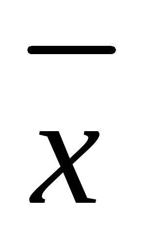 и
и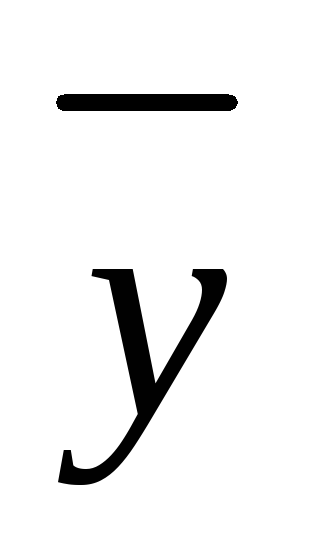 )
)
и их дисперсий (s2x
и s2y),
рассчитываемых по стандартным формулам
(см. раздел 5).
Использование критерия
Стьюдента предполагает соблюдение
следующих условий:
-
Распределения значений
для обеих выборок должны соответствовать
закону нормального распределения (см.
раздел 6). -
Суммарный объем выборок
должен быть не менее 30 (для β1
= 0,95) и не менее 100 (для β2
= 0,99). -
Объемы двух выборок
не должны существенно отличаться друг
от друга (не более чем в 1,5 ÷ 2 раза).
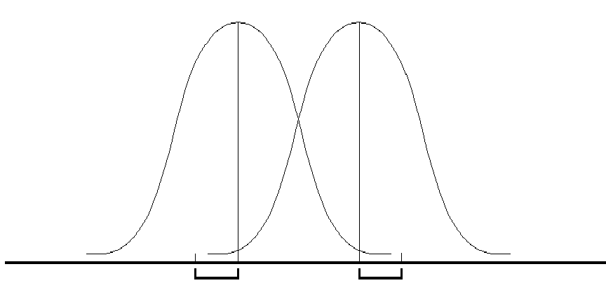
Идея критерия Стьюдента
достаточно проста. Предположим, что
значения переменных в каждой из выборок
распределяются по нормальному закону,
т. е. мы имеем дело с двумя нормальными
распределениями, отличающимися друг
от друга по средним значениям и дисперсии
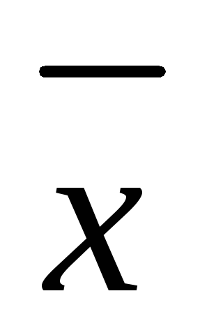
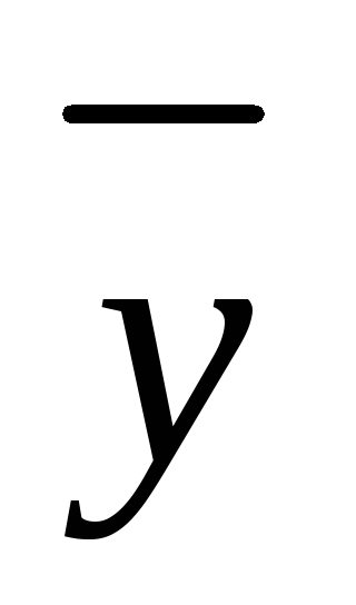
(соответственно
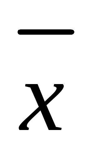 и
и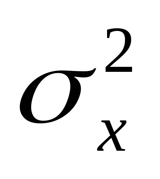 ,
,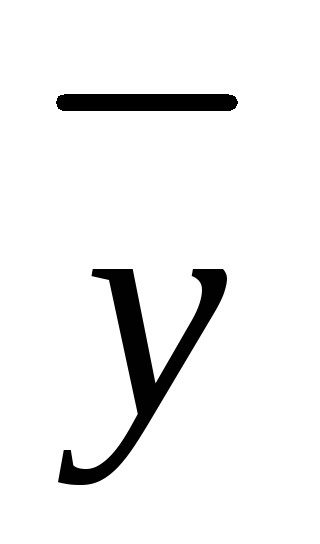 и
и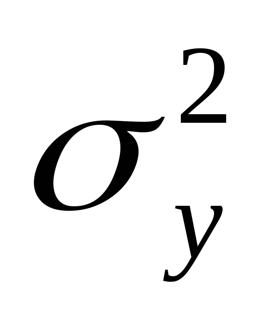 ,
,
см. рис. 7.1).
sx
 sy
sy
Рис.
7.1. Оценка различий между двумя независимыми
выборками:
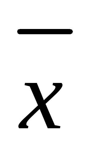 и
и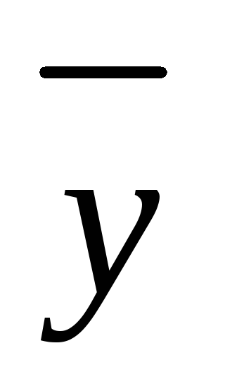 —
—
средние значения выборок x
и y;
sx
и sy
—
стандартные отклонения
Нетрудно понять, что
различия между двумя выборками будут
тем больше, чем больше разность между
средними значениями и чем меньше их
дисперсии (или стандартные отклонения).
В
случае независимых выборок коэффициент
Стьюдента определяют по формуле:
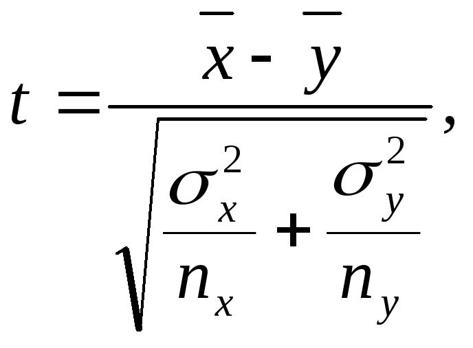 (7.2)
(7.2)
где nx
и ny
– соответственно численность выборок
x
и y.
После вычисления
коэффициента Стьюдента в таблице
стандартных (критических) значений t
(см. Приложение, табл. Х) находят величину,
соответствующую числу степеней свободы
n
= nx
+ ny
– 2, и сравнивают
ее с рассчитанной по формуле. Если tэксп.
£
tкр.,
то гипотезу о достоверности различий
между выборками отвергают, если же
tэксп.
> tкр.,
то ее принимают. Другими словами, выборки
достоверно отличаются друг от друга,
если вычисленный по формуле коэффициент
Стьюдента больше табличного значения
для соответствующего уровня значимости.
В рассмотренной нами
ранее задаче вычисление средних значений
и дисперсий дает следующие значения:
xср.
= 38,5; σх2
= 28,40; уср.
= 36,2; σу2
= 31,72.
Можно видеть, что
среднее значение тревожности в группе
девушек выше, чем в группе юношей. Тем
не менее эти различия настолько
незначительны, что вряд ли они являются
статистически значимыми. Разброс
значений у юношей, напротив, несколько
выше, чем у девушек, но различия между
дисперсиями также невелики.
Подставляем
значения в формулу:

Вывод
tэксп.
= 1,14 < tкр.
= 2,05 (β1
= 0,95). Различия между двумя сравниваемыми
выборками не являются статистически
достоверными. Данный вывод вполне
согласуется с таковым, полученным при
использовании критериев Розенбаума и
Манна-Уитни.
Другой
способ определения различий между двумя
выборками по критерию Стьюдента состоит
в вычислении доверительного интервала
стандартных отклонений. Доверительным
интервалом называется среднеквадратичное
(стандартное) отклонение, деленное на
корень квадратный из объема выборки и
умноженное на стандартное значение
коэффициента Стьюдента для n
– 1 степеней свободы (соответственно,
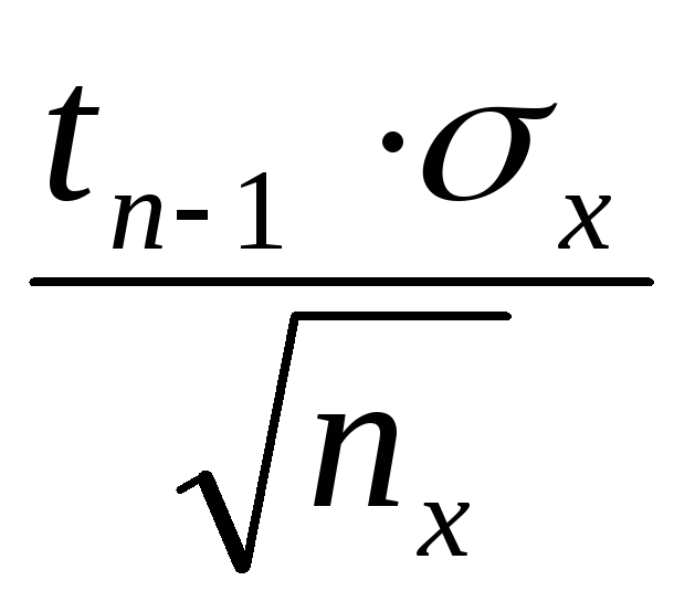 и
и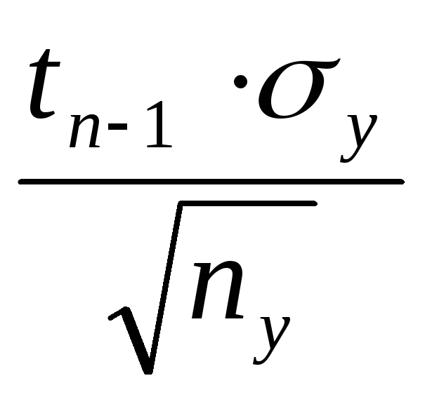 ).
).
Примечание
Величина
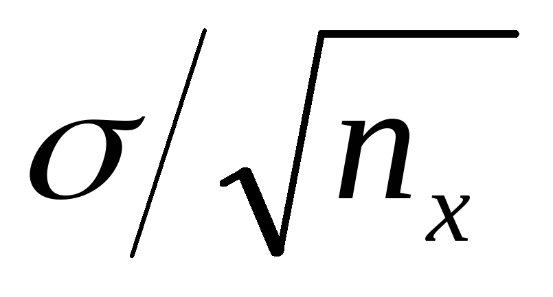 =mx
=mx
называется
среднеквадратичной ошибкой (см. раздел
5). Следовательно, доверительный интервал
есть среднеквадратичная ошибка,
умноженная на коэффициент Стьюдента
для данного объема выборки, где число
степеней свободы ν = n
– 1, и заданного уровня значимости.
Две
независимые друг от друга выборки
считаются достоверно различающимися,
если доверительные интервалы для этих
выборок не перекрываются друг с другом.
В нашем случае мы имеем для первой
выборки 38,5 ± 2,84, для второй 36,2 ± 3,38.
Следовательно,
случайные вариации xi
лежат в диапазоне 35,66 ¸
41,34, а вариации yi
– в диапазоне 32,82 ¸
39,58. На основании этого можно констатировать,
что различия между выборками x
и y
статистически недостоверны (диапазоны
вариаций перекрываются друг с другом).
При этом следует иметь в виду, что ширина
зоны перекрытия в данном случае не имеет
значения (важен лишь сам факт перекрытия
доверительных интервалов).
Метод
Стьюдента для зависимых друг от друга
выборок (например, для сравнения
результатов, полученных при повторном
тестировании на одной и той же выборке
испытуемых) используют достаточно
редко, поскольку для этих целей существуют
другие, более информативные статистические
приемы (см. раздел 10). Тем не менее, для
данной цели в первом приближении можно
использовать формулу Стьюдента следующего
вида:
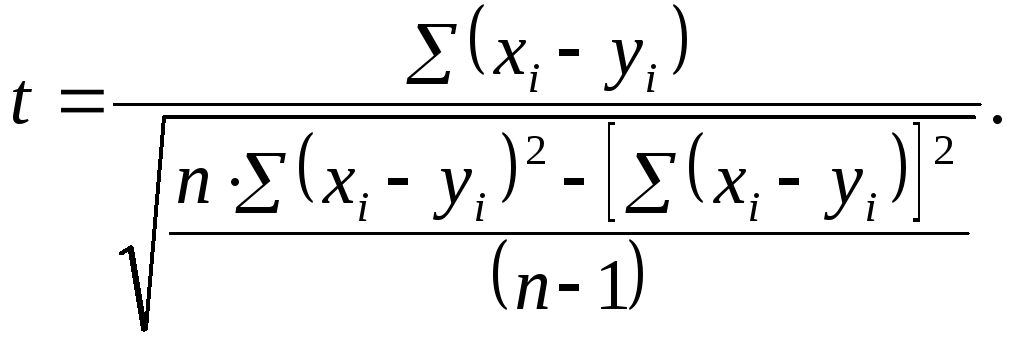 (7.3)
(7.3)
Полученный результат
сравнивают с табличным значением для
n
– 1 степеней свободы, где n
– число пар значений x
и y.
Результаты сравнения интерпретируются
точно так же, как и в случае вычисления
различий между двумя независимыми
выборками.
Соседние файлы в предмете [НЕСОРТИРОВАННОЕ]
- #
- #
23.02.201514.96 Mб37Longman_Advanced_Learners_39_Grammar.pdf
- #
- #
- #
- #
- #
- #
- #
- #
- #
Коэффициенты Стьюдента
- Коэффициенты Стьюдента
-
Кванти́ли (проценти́ли) распределе́ния Стью́дента (коэффициенты Стьюдента) — числовые характеристики, широко используемые в задачах математической статистики таких как построение доверительных интервалов и проверка статистических гипотез.
Содержание
- 1 Определение
- 2 Замечания
- 3 Таблица квантилей
- 3.1 Пример
- 4 См. также
Определение
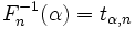
Пусть Fn — функция распределения Стьюдента t(n) с n степенями свободы, и
![alpha in [0,1]](https://dic.academic.ru/pictures/wiki/files/55/74f725ac10fd07911d173c277b58814f.png) . Тогда α-квантилью этого распределения называется число tα,n такое, что
. Тогда α-квантилью этого распределения называется число tα,n такое, что .
.
Замечания
 .
.
- Функция
 не имеет простого представления. Однако, возможно вычислить её значения численно.
 - Распределение t(n) симметрично. Следовательно,
- t1 − α,n = − tα,n.
Таблица квантилей
Нижеприведённая таблица получена с помощью функции tinv пакета tα,n, необходимо найти строку, соответствующую нужному n, и колонку, соответствующую нужному α. Искомое число находится в таблице на их пересечении.
Пример
- t0.2,4 = 0.2707;
- t0.8,4 = − t0.2,4 = − 0.2707.
См. также
- Распределение Стьюдента;
- Доверительный интервал для математического ожидания нормальной выборки.
Квантили tα,n
two-tailed test 1-0.9/2 1-0.8/2 1-0.7/2 1-0.6/2 1-0.5/2 1-0.4/2 1-0.3/2 1-0.2/2 1-0.1/2 1-0.05/2 1-0.02/2 one-tailed test 1-0.9 1-0.8 1-0.7 1-0.6 1-0.5 1-0.4 1-0.3 1-0.2 1-0.1 1-0.05 1-0.02 1 0.1584 0.3249 0.5095 0.7265 1.0000 1.3764 1.9626 3.0777 6.3138 12.7062 31.8205 2 0.1421 0.2887 0.4447 0.6172 0.8165 1.0607 1.3862 1.8856 2.9200 4.3027 6.9646 3 0.1366 0.2767 0.4242 0.5844 0.7649 0.9785 1.2498 1.6377 2.3534 3.1824 4.5407 4 0.1338 0.2707 0.4142 0.5686 0.7407 0.9410 1.1896 1.5332 2.1318 2.7764 3.7469 5 0.1322 0.2672 0.4082 0.5594 0.7267 0.9195 1.1558 1.4759 2.0150 2.5706 3.3649 6 0.1311 0.2648 0.4043 0.5534 0.7176 0.9057 1.1342 1.4398 1.9432 2.4469 3.1427 7 0.1303 0.2632 0.4015 0.5491 0.7111 0.8960 1.1192 1.4149 1.8946 2.3646 2.9980 8 0.1297 0.2619 0.3995 0.5459 0.7064 0.8889 1.1081 1.3968 1.8595 2.3060 2.8965 9 0.1293 0.2610 0.3979 0.5435 0.7027 0.8834 1.0997 1.3830 1.8331 2.2622 2.8214 10 0.1289 0.2602 0.3966 0.5415 0.6998 0.8791 1.0931 1.3722 1.8125 2.2281 2.7638 11 0.1286 0.2596 0.3956 0.5399 0.6974 0.8755 1.0877 1.3634 1.7959 2.2010 2.7181 12 0.1283 0.2590 0.3947 0.5386 0.6955 0.8726 1.0832 1.3562 1.7823 2.1788 2.6810 13 0.1281 0.2586 0.3940 0.5375 0.6938 0.8702 1.0795 1.3502 1.7709 2.1604 2.6503 14 0.1280 0.2582 0.3933 0.5366 0.6924 0.8681 1.0763 1.3450 1.7613 2.1448 2.6245 15 0.1278 0.2579 0.3928 0.5357 0.6912 0.8662 1.0735 1.3406 1.7531 2.1314 2.6025 16 0.1277 0.2576 0.3923 0.5350 0.6901 0.8647 1.0711 1.3368 1.7459 2.1199 2.5835 17 0.1276 0.2573 0.3919 0.5344 0.6892 0.8633 1.0690 1.3334 1.7396 2.1098 2.5669 18 0.1274 0.2571 0.3915 0.5338 0.6884 0.8620 1.0672 1.3304 1.7341 2.1009 2.5524 19 0.1274 0.2569 0.3912 0.5333 0.6876 0.8610 1.0655 1.3277 1.7291 2.0930 2.5395 20 0.1273 0.2567 0.3909 0.5329 0.6870 0.8600 1.0640 1.3253 1.7247 2.0860 2.5280 21 0.1272 0.2566 0.3906 0.5325 0.6864 0.8591 1.0627 1.3232 1.7207 2.0796 2.5176 22 0.1271 0.2564 0.3904 0.5321 0.6858 0.8583 1.0614 1.3212 1.7171 2.0739 2.5083 23 0.1271 0.2563 0.3902 0.5317 0.6853 0.8575 1.0603 1.3195 1.7139 2.0687 2.4999 24 0.1270 0.2562 0.3900 0.5314 0.6848 0.8569 1.0593 1.3178 1.7109 2.0639 2.4922 25 0.1269 0.2561 0.3898 0.5312 0.6844 0.8562 1.0584 1.3163 1.7081 2.0595 2.4851 26 0.1269 0.2560 0.3896 0.5309 0.6840 0.8557 1.0575 1.3150 1.7056 2.0555 2.4786 27 0.1268 0.2559 0.3894 0.5306 0.6837 0.8551 1.0567 1.3137 1.7033 2.0518 2.4727 28 0.1268 0.2558 0.3893 0.5304 0.6834 0.8546 1.0560 1.3125 1.7011 2.0484 2.4671 29 0.1268 0.2557 0.3892 0.5302 0.6830 0.8542 1.0553 1.3114 1.6991 2.0452 2.4620 30 0.1267 0.2556 0.3890 0.5300 0.6828 0.8538 1.0547 1.3104 1.6973 2.0423 2.4573 31 0.1267 0.2555 0.3889 0.5298 0.6825 0.8534 1.0541 1.3095 1.6955 2.0395 2.4528 32 0.1267 0.2555 0.3888 0.5297 0.6822 0.8530 1.0535 1.3086 1.6939 2.0369 2.4487 33 0.1266 0.2554 0.3887 0.5295 0.6820 0.8526 1.0530 1.3077 1.6924 2.0345 2.4448 34 0.1266 0.2553 0.3886 0.5294 0.6818 0.8523 1.0525 1.3070 1.6909 2.0322 2.4411 35 0.1266 0.2553 0.3885 0.5292 0.6816 0.8520 1.0520 1.3062 1.6896 2.0301 2.4377 36 0.1266 0.2552 0.3884 0.5291 0.6814 0.8517 1.0516 1.3055 1.6883 2.0281 2.4345 37 0.1265 0.2552 0.3883 0.5289 0.6812 0.8514 1.0512 1.3049 1.6871 2.0262 2.4314 38 0.1265 0.2551 0.3882 0.5288 0.6810 0.8512 1.0508 1.3042 1.6860 2.0244 2.4286 39 0.1265 0.2551 0.3882 0.5287 0.6808 0.8509 1.0504 1.3036 1.6849 2.0227 2.4258 40 0.1265 0.2550 0.3881 0.5286 0.6807 0.8507 1.0500 1.3031 1.6839 2.0211 2.4233 41 0.1264 0.2550 0.3880 0.5285 0.6805 0.8505 1.0497 1.3025 1.6829 2.0195 2.4208 42 0.1264 0.2550 0.3880 0.5284 0.6804 0.8503 1.0494 1.3020 1.6820 2.0181 2.4185 43 0.1264 0.2549 0.3879 0.5283 0.6802 0.8501 1.0491 1.3016 1.6811 2.0167 2.4163 44 0.1264 0.2549 0.3878 0.5282 0.6801 0.8499 1.0488 1.3011 1.6802 2.0154 2.4141 45 0.1264 0.2549 0.3878 0.5281 0.6800 0.8497 1.0485 1.3006 1.6794 2.0141 2.4121 46 0.1264 0.2548 0.3877 0.5281 0.6799 0.8495 1.0483 1.3002 1.6787 2.0129 2.4102 47 0.1263 0.2548 0.3877 0.5280 0.6797 0.8493 1.0480 1.2998 1.6779 2.0117 2.4083 48 0.1263 0.2548 0.3876 0.5279 0.6796 0.8492 1.0478 1.2994 1.6772 2.0106 2.4066 49 0.1263 0.2547 0.3876 0.5278 0.6795 0.8490 1.0475 1.2991 1.6766 2.0096 2.4049 50 0.1263 0.2547 0.3875 0.5278 0.6794 0.8489 1.0473 1.2987 1.6759 2.0086 2.4033 100 0.1260 0.2540 0.3864 0.5261 0.6770 0.8452 1.0418 1.2901 1.6602 1.9840 2.3642 1000 0.1257 0.2534 0.3854 0.5246 0.6747 0.8420 1.0370 1.2824 1.6464 1.9623 2.3301
Wikimedia Foundation.
2010.
Полезное
Смотреть что такое «Коэффициенты Стьюдента» в других словарях:
-
Процентили распределения Стьюдента — Квантили (процентили) распределения Стьюдента (коэффициенты Стьюдента) числовые характеристики, широко используемые в задачах математической статистики таких как построение доверительных интервалов и проверка статистических гипотез. Содержание 1 … Википедия
-
Квантили распределения Стьюдента — Квантили (процентили) распределения Стьюдента (коэффициенты Стьюдента) числовые характеристики, широко используемые в задачах математической статистики таких как построение доверительных интервалов и проверка статистических гипотез.… … Википедия
-
Коэффициент корреляции — (Correlation coefficient) Коэффициент корреляции это статистический показатель зависимости двух случайных величин Определение коэффициента корреляции, виды коэффициентов корреляции, свойства коэффициента корреляции, вычисление и применение… … Энциклопедия инвестора
-
Корреляция — (Correlation) Корреляция это статистическая взаимосвязь двух или нескольких случайных величин Понятие корреляции, виды корреляции, коэффициент корреляции, корреляционный анализ, корреляция цен, корреляция валютных пар на Форекс Содержание… … Энциклопедия инвестора
-
Наименьших квадратов метод — один из методов ошибок теории (См. Ошибок теория) для оценки неизвестных величин по результатам измерений, содержащим случайные ошибки. Н. к. м. применяется также для приближённого представления заданной функции другими (более простыми)… … Большая советская энциклопедия
-
Математи́ческие ме́тоды — в медицине совокупность методов количественного изучения и анализа состояния и (или) поведения объектов и систем, относящихся к медицине и здравоохранению. В биологии, медицине и здравоохранении в круг явлений, изучаемых с помощью М.м., входят… … Медицинская энциклопедия
-
НАИМЕНЬШИХ КВАДРАТОВ МЕТОД — один из методов ошибок теории для оценки неизвестных величин по результатам измерений, содержащим случайные ошибки. Н. к. м. применяется также для приближенного представления заданной функции другими (более простыми) функциями и часто оказывается … Математическая энциклопедия
-
РДМУ 109-77: Методические указания. Методика выбора и оптимизации контролируемых параметров технологических процессов — Терминология РДМУ 109 77: Методические указания. Методика выбора и оптимизации контролируемых параметров технологических процессов: 73. Адекватность модели Соответствие модели с экспериментальными данными по выбранному параметру оптимизации с… … Словарь-справочник терминов нормативно-технической документации
-
ГОСТ Р 50779.10-2000: Статистические методы. Вероятность и основы статистики. Термины и определения — Терминология ГОСТ Р 50779.10 2000: Статистические методы. Вероятность и основы статистики. Термины и определения оригинал документа: 2.3. (генеральная) совокупность Множество всех рассматриваемых единиц. Примечание Для случайной величины… … Словарь-справочник терминов нормативно-технической документации
-
Нахождение дисперсии ошибки определения коэффициента регрессии — 3.9.3. Нахождение дисперсии ошибки определения коэффициента регрессии При равном числе параллельных опытов (m0) во всех точках плана матрицы дисперсию ошибки определения коэффициента регрессии определяют по формуле… … Словарь-справочник терминов нормативно-технической документации
Доверительные интервалы
Общий обзор
Доверительный интервал для среднего
Доверительный интервал для пропорции
Интерпретация доверительных интервалов
Общий обзор
Взяв выборку из популяции, мы получим точечную оценку интересующего нас параметра и вычислим стандартную ошибку для того, чтобы указать точность оценки.
Однако, для большинства случаев стандартная ошибка как такова не приемлема. Гораздо полезнее объединить эту меру точности с интервальной оценкой для параметра популяции.
Это можно сделать, используя знания о теоретическом распределении вероятности выборочной статистики (параметра) для того, чтобы вычислить доверительный интервал (CI – Confidence Interval, ДИ – Доверительный интервал) для параметра.
Вообще, доверительный интервал расширяет оценки в обе стороны некоторой величиной, кратной стандартной ошибке (данного параметра); два значения (доверительные границы), определяющие интервал, обычно отделяют запятой и заключают в скобки.
Доверительный интервал для среднего
Использование нормального распределения
Выборочное среднее  имеет нормальное распределение, если объем выборки большой, поэтому можно применить знания о нормальном распределении при рассмотрении выборочного среднего.
В частности, 95% распределения выборочных средних находится в пределах 1,96 стандартных отклонений (SD) среднего популяции.
Когда у нас есть только одна выборка, мы называем это стандартной ошибкой среднего (SEM) и вычисляем 95% доверительного интервала для среднего следующим образом:

Если повторить этот эксперимент несколько раз, то интервал будет содержать истинное среднее популяции в 95% случаев.
Обычно это доверительный интервал как, например, интервал значений, в пределах которого с доверительной вероятностью 95% находится истинное среднее популяции (генеральное среднее).
Хотя это не вполне строго (среднее в популяции есть фиксированное значение и поэтому не может иметь вероятность, отнесённую к нему) таким образом интерпретировать доверительный интервал, но концептуально это удобнее для понимания.
Использование t-распределения
Можно использовать нормальное распределение, если знать значение дисперсии в популяции. Кроме того, когда объем выборки небольшой, выборочное среднее отвечает нормальному распределению, если данные, лежащие в основе популяции, распределены нормально.
Если данные, лежащие в основе популяции, распределены ненормально и/или неизвестна генеральная дисперсия (дисперсия в популяции), выборочное среднее подчиняется t-распределению Стьюдента.
Вычисляем 95% доверительный интервал для генерального среднего в популяции следующим образом:

где  — процентная точка (процентиль) t-распределения Стьюдента с (n-1) степенями свободы, которая даёт двухстороннюю вероятность 0,05.
Вообще, она обеспечивает более широкий интервал, чем при использовании нормального распределения, поскольку учитывает дополнительную неопределенность, которую вводят, оценивая стандартное отклонение популяции и/или из-за небольшого объёма выборки.
Когда объём выборки большой (порядка 100 и более), разница между двумя распределениями (t-Стьюдента и нормальным) незначительна. Тем не менее всегда используют t-распределение при вычислении доверительных интервалов, даже если объем выборки большой.
Обычно указывают 95% ДИ. Можно вычислить другие доверительные интервалы, например 99% ДИ для среднего.
Вместо произведения стандартной ошибки и табличного значения t-распределения, которое соответствует двусторонней вероятности 0,05, умножают её (стандартную ошибку) на значение, которое соответствует двусторонней вероятности 0,01. Это более широкий доверительный интервал, чем в случае 95%, поскольку он отражает увеличенное доверие к тому, что интервал действительно включает среднее популяции.
Доверительный интервал для пропорции
Выборочное распределение пропорций имеет биномиальное распределение. Однако если объём выборки n разумно большой, тогда выборочное распределение пропорции приблизительно нормально со средним  .
.
Оцениваем выборочным отношением p=r/n (где r– количество индивидуумов в выборке с интересующими нас характерными особенностями), и стандартная ошибка оценивается:

95% доверительный интервал для пропорции оценивается:

Если объём выборки небольшой (обычно когда np или n(1-p) меньше 5), тогда необходимо использовать биномиальное распределение для того, чтобы вычислить точные доверительные интервалы.
Заметьте, что если p выражается в процентах, то (1-p) заменяют на (100-p).
Интерпретация доверительных интервалов
При интерпретации доверительного интервала нас интересуют следующие вопросы:
Насколько широк доверительный интервал?
Широкий доверительный интервал указывает на то, что оценка неточна; узкий указывает на точную оценку.
Ширина доверительного интервала зависит от размера стандартной ошибки, которая, в свою очередь, зависит от объёма выборки и при рассмотрении числовой переменной от изменчивости данных дают более широкие доверительные интервалы, чем исследования многочисленного набора данных немногих переменных.
Включает ли ДИ какие-либо значения, представляющие особенный интерес?
Можно проверить, ложится ли вероятное значение для параметра популяции в пределы доверительного интервала. Если да, то результаты согласуются с этим вероятным значением. Если нет, тогда маловероятно (для 95% доверительного интервала шанс почти 5%), что параметр имеет это значение.
Связанные определения:
Доверительный интервал
Доверительный предел
Коэффициент доверия
Оценка
Оценочная функция
Свободный от распределения доверительный интервал
В начало
Содержание портала
This article is about the mathematics of Student’s t-distribution. For its uses in statistics, see Student’s t-test.
|
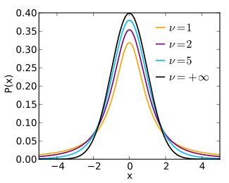
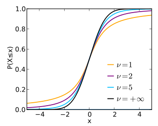
Probability density function
|
|
|
Cumulative distribution function
|
|
| Parameters |
 degrees of freedom (real) degrees of freedom (real) |
|---|---|
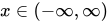
| Support |
 |
 |
|
| CDF |
where 2F1 is the hypergeometric function |
| Mean |
0 for  , otherwise undefined , otherwise undefined |
| Median | 0 |
| Mode | 0 |
| Variance |
 for for  , ∞ for , ∞ for  , otherwise undefined , otherwise undefined |
| Skewness |
0 for  , otherwise undefined , otherwise undefined |
| Ex. kurtosis |
 for for  , ∞ for , ∞ for  , otherwise undefined , otherwise undefined |
| Entropy |
|
| MGF | undefined |
| CF |
|
![begin{matrix}
frac{1}{2} + x Gamma left( frac{nu+1}{2} right) times\[0.5em]
frac{,_2F_1 left ( frac{1}{2},frac{nu+1}{2};frac{3}{2};
-frac{x^2}{nu} right)}
{sqrt{pinu},Gamma left(frac{nu}{2}right)}
end{matrix}](https://wikimedia.org/api/rest_v1/media/math/render/svg/7c3c84e8f1257dce799724d08e3b08389944045d)
![{displaystyle {begin{matrix}{frac {nu +1}{2}}left[psi left({frac {1+nu }{2}}right)-psi left({frac {nu }{2}}right)right]\[0.5em]+ln {left[{sqrt {nu }}Bleft({frac {nu }{2}},{frac {1}{2}}right)right]},{scriptstyle {text{(nats)}}}end{matrix}}}](https://wikimedia.org/api/rest_v1/media/math/render/svg/8e64e6a7fd1bb08a7129701a00f10b4dc673c589)

In probability and statistics, Student’s t-distribution (or simply the t-distribution) is any member of a family of continuous probability distributions that arise when estimating the mean of a normally distributed population in situations where the sample size is small and the population’s standard deviation is unknown. It was developed by English statistician William Sealy Gosset under the pseudonym «Student».
The t-distribution plays a role in a number of widely used statistical analyses, including Student’s t-test for assessing the statistical significance of the difference between two sample means, the construction of confidence intervals for the difference between two population means, and in linear regression analysis. Student’s t-distribution also arises in the Bayesian analysis of data from a normal family.
If we take a sample of 


The t-distribution is symmetric and bell-shaped, like the normal distribution. However, the t-distribution has heavier tails, meaning that it is more prone to producing values that fall far from its mean. This makes it useful for understanding the statistical behavior of certain types of ratios of random quantities, in which variation in the denominator is amplified and may produce outlying values when the denominator of the ratio falls close to zero. The Student’s t-distribution is a special case of the generalized hyperbolic distribution.
History and etymology[edit]
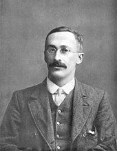
Statistician William Sealy Gosset, known as «Student»
In statistics, the t-distribution was first derived as a posterior distribution in 1876 by Helmert[2][3][4] and Lüroth.[5][6][7] The t-distribution also appeared in a more general form as Pearson Type IV distribution in Karl Pearson’s 1895 paper.[8]
In the English-language literature, the distribution takes its name from William Sealy Gosset’s 1908 paper in Biometrika under the pseudonym «Student».[9] One version of the origin of the pseudonym is that Gosset’s employer preferred staff to use pen names when publishing scientific papers instead of their real name, so he used the name «Student» to hide his identity. Another version is that Guinness did not want their competitors to know that they were using the t-test to determine the quality of raw material.[10][11]
Gosset worked at the Guinness Brewery in Dublin, Ireland, and was interested in the problems of small samples – for example, the chemical properties of barley where sample sizes might be as few as 3. Gosset’s paper refers to the distribution as the «frequency distribution of standard deviations of samples drawn from a normal population». It became well known through the work of Ronald Fisher, who called the distribution «Student’s distribution» and represented the test value with the letter t.[12][13]
How Student’s distribution arises from sampling[edit]
Let 


Let
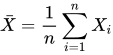
be the sample mean and let
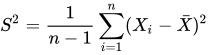
be the (Bessel-corrected) sample variance. Then the random variable

has a standard normal distribution (i.e. normal with expected mean 0 and variance 1), and the random variable

i.e where 





Definition[edit]
Probability density function[edit]
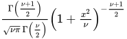
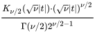
Student’s t-distribution has the probability density function (PDF) given by
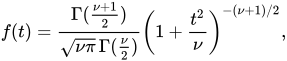
where 

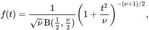
where B is the Beta function. In particular for integer valued degrees of freedom
For

For

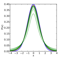
The probability density function is symmetric, and its overall shape resembles the bell shape of a normally distributed variable with mean 0 and variance 1, except that it is a bit lower and wider. As the number of degrees of freedom grows, the t-distribution approaches the normal distribution with mean 0 and variance 1. For this reason 
The following images show the density of the t-distribution for increasing values of

1 degree of freedom

2 degrees of freedom

3 degrees of freedom

5 degrees of freedom
10 degrees of freedom

30 degrees of freedom
Cumulative distribution function[edit]
The cumulative distribution function (CDF) can be written in terms of I, the regularized
incomplete beta function. For t > 0,[15]

where
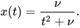
Other values would be obtained by symmetry. An alternative formula, valid for 

where 2F1 is a particular case of the hypergeometric function.
For information on its inverse cumulative distribution function, see quantile function § Student’s t-distribution.
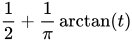
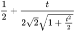
Special cases[edit]
Certain values of
|
|
CDF | notes | |
|---|---|---|---|
| 1 | 
|
|
See Cauchy distribution |
| 2 | 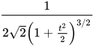
|
|
|
| 3 | 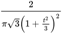
|
![{displaystyle {frac {1}{2}}+{frac {1}{pi }}{left[{frac {1}{sqrt {3}}}{frac {t}{1+{frac {t^{2}}{3}}}}+arctan left({frac {t}{sqrt {3}}}right)right]}}](https://wikimedia.org/api/rest_v1/media/math/render/svg/f0afffc07f0c86a59eaa560dc8a3cf8f6fa83ccd)
|
|
| 4 | 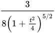
|
![{displaystyle {frac {1}{2}}+{frac {3}{8}}{frac {t}{sqrt {1+{frac {t^{2}}{4}}}}}{left[1-{frac {1}{12}}{frac {t^{2}}{1+{frac {t^{2}}{4}}}}right]}}](https://wikimedia.org/api/rest_v1/media/math/render/svg/8267697404a72109b22e9add73ef7023d1953235)
|
|
| 5 | 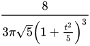
|
![{displaystyle {frac {1}{2}}+{frac {1}{pi }}{left[{frac {t}{{sqrt {5}}left(1+{frac {t^{2}}{5}}right)}}left(1+{frac {2}{3left(1+{frac {t^{2}}{5}}right)}}right)+arctan left({frac {t}{sqrt {5}}}right)right]}}](https://wikimedia.org/api/rest_v1/media/math/render/svg/aeef99bb2df092bdcc8c708cbc0c29cfe1849232)
|
|

|

|
![{displaystyle {frac {1}{2}}{left[1+operatorname {erf} left({frac {t}{sqrt {2}}}right)right]}}](https://wikimedia.org/api/rest_v1/media/math/render/svg/e86c11ecfcdc01d2a24c4afd9b4e0e0a4aff6424)
|
See Normal distribution, Error function |
How the t-distribution arises[edit]
Sampling distribution[edit]
Let 
![{displaystyle {begin{aligned}{bar {x}}&={frac {x_{1}+cdots +x_{n}}{n}},\[5pt]s^{2}&={frac {1}{n-1}}sum _{i=1}^{n}(x_{i}-{bar {x}})^{2}.end{aligned}}}](https://wikimedia.org/api/rest_v1/media/math/render/svg/3b254594b738c8226106dced8dcc81c7f7c4d2ae)
The resulting t-value is

The t-distribution with 
Bayesian inference[edit]
In Bayesian statistics, a (scaled, shifted) t-distribution arises as the marginal distribution of the unknown mean of a normal distribution, when the dependence on an unknown variance has been marginalized out:[16]
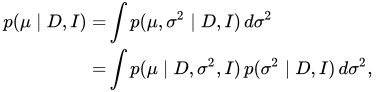
where 


With 


a normal distribution and a scaled inverse chi-squared distribution respectively, where
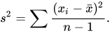
The marginalization integral thus becomes

This can be evaluated by substituting 

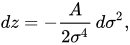
so

But the z integral is now a standard Gamma integral, which evaluates to a constant, leaving
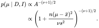
This is a form of the t-distribution with an explicit scaling and shifting that will be explored in more detail in a further section below. It can be related to the standardized t-distribution by the substitution

The derivation above has been presented for the case of uninformative priors for 

Characterization[edit]
As the distribution of a test statistic[edit]
Student’s t-distribution with
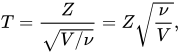
where
- Z is a standard normal with expected value 0 and variance 1;
- V has a chi-squared distribution (χ2-distribution) with
- Z and V are independent;
A different distribution is defined as that of the random variable defined, for a given constant μ, by
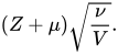
This random variable has a noncentral t-distribution with noncentrality parameter μ. This distribution is important in studies of the power of Student’s t-test.
Derivation[edit]
Suppose X1, …, Xn are independent realizations of the normally-distributed, random variable X, which has an expected value μ and variance σ2. Let
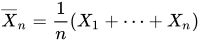
be the sample mean, and
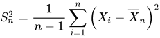
be an unbiased estimate of the variance from the sample. It can be shown that the random variable
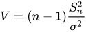
has a chi-squared distribution with
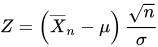
is normally distributed with mean 0 and variance 1, since the sample mean 

which differs from Z in that the exact standard deviation σ is replaced by the random variable Sn, has a Student’s t-distribution as defined above. Notice that the unknown population variance σ2 does not appear in T, since it was in both the numerator and the denominator, so it canceled. Gosset intuitively obtained the probability density function stated above, with
The distribution of the test statistic T depends on
As a maximum entropy distribution[edit]
Student’s t-distribution is the maximum entropy probability distribution for a random variate X for which 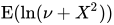
Properties[edit]
Moments[edit]
For
![{displaystyle operatorname {E} (T^{k})={begin{cases}0&k{text{ odd}},quad 0<k<nu \{frac {1}{{sqrt {pi }}Gamma left({frac {nu }{2}}right)}}left[Gamma left({frac {k+1}{2}}right)Gamma left({frac {nu -k}{2}}right)nu ^{frac {k}{2}}right]&k{text{ even}},quad 0<k<nu .\end{cases}}}](https://wikimedia.org/api/rest_v1/media/math/render/svg/876ddf907881d570498829eb97d785812295cf58)
Moments of order
The term for 

For a t-distribution with 

Monte Carlo sampling[edit]
There are various approaches to constructing random samples from the Student’s t-distribution. The matter depends on whether the samples are required on a stand-alone basis, or are to be constructed by application of a quantile function to uniform samples; e.g., in the multi-dimensional applications basis of copula-dependency.[citation needed] In the case of stand-alone sampling, an extension of the Box–Muller method and its polar form is easily deployed.[21] It has the merit that it applies equally well to all real positive degrees of freedom, ν, while many other candidate methods fail if ν is close to zero.[21]
Integral of Student’s probability density function and p-value[edit]
The function A(t | ν) is the integral of Student’s probability density function, f(t) between −t and t, for t ≥ 0. It thus gives the probability that a value of t less than that calculated from observed data would occur by chance. Therefore, the function A(t | ν) can be used when testing whether the difference between the means of two sets of data is statistically significant, by calculating the corresponding value of t and the probability of its occurrence if the two sets of data were drawn from the same population. This is used in a variety of situations, particularly in t-tests. For the statistic t, with ν degrees of freedom, A(t | ν) is the probability that t would be less than the observed value if the two means were the same (provided that the smaller mean is subtracted from the larger, so that t ≥ 0). It can be easily calculated from the cumulative distribution function Fν(t) of the t-distribution:

where Ix is the regularized incomplete beta function (a, b).
For statistical hypothesis testing this function is used to construct the p-value.
Generalized Student’s t-distribution[edit]
In terms of scaling parameter σ̂ or σ̂2[edit]
Student’s t distribution can be generalized to a three parameter location-scale family, introducing a location parameter 


or

This means that 
The resulting non-standardized Student’s t-distribution has a density defined by:[22]

Here, 
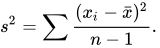
Equivalently, the distribution can be written in terms of 

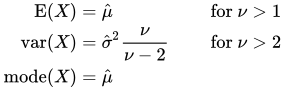
Other properties of this version of the distribution are:[22]
This distribution results from compounding a Gaussian distribution (normal distribution) with mean 

Equivalently, this distribution results from compounding a Gaussian distribution with a scaled-inverse-chi-squared distribution with parameters 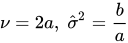
This version of the t-distribution can be useful in financial modeling. For example, Platen and Sidorowicz found that among the family of generalized hyperbolic distributions, this form of the t-distribution with about 4 degrees of freedom was the best fit for the (log) return of many worldwide stock indices.[23]
In terms of inverse scaling parameter λ[edit]
An alternative parameterization in terms of an inverse scaling parameter 


Other properties of this version of the distribution are:[24]
![{displaystyle {begin{aligned}operatorname {E} (X)&={hat {mu }}&&{text{ for }}nu >1\[5pt]operatorname {var} (X)&={frac {1}{lambda }}{frac {nu }{nu -2}}&&{text{ for }}nu >2\[5pt]operatorname {mode} (X)&={hat {mu }}end{aligned}}}](https://wikimedia.org/api/rest_v1/media/math/render/svg/5d718430b8350f0ada28d216c96d8944e72d7e2a)
This distribution results from compounding a Gaussian distribution with mean 
[edit]
- If
has a Student’s t-distribution with degree of freedom
- The noncentral t-distribution generalizes the t-distribution to include a location parameter. Unlike the nonstandardized t-distributions, the noncentral distributions are not symmetric (the median is not the same as the mode).
- The discrete Student’s t-distribution is defined by its probability mass function at r being proportional to:[25]
Here a, b, and k are parameters. This distribution arises from the construction of a system of discrete distributions similar to that of the Pearson distributions for continuous distributions.[26]
- One can generate Student-t samples by taking the ratio of variables from the normal distribution and the square-root of χ2-distribution. If we use instead of the normal distribution, e.g., the Irwin–Hall distribution, we obtain over-all a symmetric 4-parameter distribution, which includes the normal, the uniform, the triangular, the Student-t and the Cauchy distribution. This is also more flexible than some other symmetric generalizations of the normal distribution.
- t-distribution is an instance of ratio distributions.


Bayesian inference: prior distribution for the degrees of the freedom[edit]
Suppose that 


With a choice a prior for the degrees of freedom 


Mean squared error comparison between Bayes estimators based on the four priors and maximum likelihood estimator for the degrees of the freedom. Data is simulated from the student t distribution with the degrees of freedom 


Some popular choices of the priors are:
- Jeffreys prior [28]
where 

- Exponential prior [29]

- Gamma prior [30]

- Log-normal prior [31]
![{displaystyle pi _{L}(nu )=logN(nu |1,1)={frac {1}{nu {sqrt {2pi }}}}exp left[-{frac {(log nu -1)^{2}}{2}}right],quad nu in mathbb {R} ^{+}}](https://wikimedia.org/api/rest_v1/media/math/render/svg/2286de11b6b2ca854ad197e07212694e467d1dea)
The right panels show the result of the numerical experiments. The Bayes estimator based on the Jeffreys prior 


Uses[edit]
In frequentist statistical inference[edit]
Student’s t-distribution arises in a variety of statistical estimation problems where the goal is to estimate an unknown parameter, such as a mean value, in a setting where the data are observed with additive errors. If (as in nearly all practical statistical work) the population standard deviation of these errors is unknown and has to be estimated from the data, the t-distribution is often used to account for the extra uncertainty that results from this estimation. In most such problems, if the standard deviation of the errors were known, a normal distribution would be used instead of the t-distribution.
Confidence intervals and hypothesis tests are two statistical procedures in which the quantiles of the sampling distribution of a particular statistic (e.g. the standard score) are required. In any situation where this statistic is a linear function of the data, divided by the usual estimate of the standard deviation, the resulting quantity can be rescaled and centered to follow Student’s t-distribution. Statistical analyses involving means, weighted means, and regression coefficients all lead to statistics having this form.
Quite often, textbook problems will treat the population standard deviation as if it were known and thereby avoid the need to use the Student’s t-distribution. These problems are generally of two kinds: (1) those in which the sample size is so large that one may treat a data-based estimate of the variance as if it were certain, and (2) those that illustrate mathematical reasoning, in which the problem of estimating the standard deviation is temporarily ignored because that is not the point that the author or instructor is then explaining.
Hypothesis testing[edit]
A number of statistics can be shown to have t-distributions for samples of moderate size under null hypotheses that are of interest, so that the t-distribution forms the basis for significance tests. For example, the distribution of Spearman’s rank correlation coefficient ρ, in the null case (zero correlation) is well approximated by the t distribution for sample sizes above about 20.[citation needed]
Confidence intervals[edit]
Suppose the number A is so chosen that

when T has a t-distribution with n − 1 degrees of freedom. By symmetry, this is the same as saying that A satisfies

so A is the «95th percentile» of this probability distribution, or 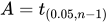
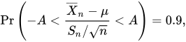
and this is equivalent to

Therefore, the interval whose endpoints are

is a 90% confidence interval for μ. Therefore, if we find the mean of a set of observations that we can reasonably expect to have a normal distribution, we can use the t-distribution to examine whether the confidence limits on that mean include some theoretically predicted value – such as the value predicted on a null hypothesis.
It is this result that is used in the Student’s t-tests: since the difference between the means of samples from two normal distributions is itself distributed normally, the t-distribution can be used to examine whether that difference can reasonably be supposed to be zero.
If the data are normally distributed, the one-sided (1 − α)-upper confidence limit (UCL) of the mean, can be calculated using the following equation:
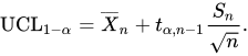
The resulting UCL will be the greatest average value that will occur for a given confidence interval and population size. In other words,
Prediction intervals[edit]
The t-distribution can be used to construct a prediction interval for an unobserved sample from a normal distribution with unknown mean and variance.
In Bayesian statistics[edit]
The Student’s t-distribution, especially in its three-parameter (location-scale) version, arises frequently in Bayesian statistics as a result of its connection with the normal distribution. Whenever the variance of a normally distributed random variable is unknown and a conjugate prior placed over it that follows an inverse gamma distribution, the resulting marginal distribution of the variable will follow a Student’s t-distribution. Equivalent constructions with the same results involve a conjugate scaled-inverse-chi-squared distribution over the variance, or a conjugate gamma distribution over the precision. If an improper prior proportional to σ−2 is placed over the variance, the t-distribution also arises. This is the case regardless of whether the mean of the normally distributed variable is known, is unknown distributed according to a conjugate normally distributed prior, or is unknown distributed according to an improper constant prior.
Related situations that also produce a t-distribution are:
- The marginal posterior distribution of the unknown mean of a normally distributed variable, with unknown prior mean and variance following the above model.
- The prior predictive distribution and posterior predictive distribution of a new normally distributed data point when a series of independent identically distributed normally distributed data points have been observed, with prior mean and variance as in the above model.
Robust parametric modeling[edit]
The t-distribution is often used as an alternative to the normal distribution as a model for data, which often has heavier tails than the normal distribution allows for; see e.g. Lange et al.[32] The classical approach was to identify outliers (e.g., using Grubbs’s test) and exclude or downweight them in some way. However, it is not always easy to identify outliers (especially in high dimensions), and the t-distribution is a natural choice of model for such data and provides a parametric approach to robust statistics.
A Bayesian account can be found in Gelman et al.[33] The degrees of freedom parameter controls the kurtosis of the distribution and is correlated with the scale parameter. The likelihood can have multiple local maxima and, as such, it is often necessary to fix the degrees of freedom at a fairly low value and estimate the other parameters taking this as given. Some authors[citation needed] report that values between 3 and 9 are often good choices. Venables and Ripley[citation needed] suggest that a value of 5 is often a good choice.
Student’s t-process[edit]
For practical regression and prediction needs, Student’s t-processes were introduced, that are generalisations of the Student t-distributions for functions. A Student’s t-process is constructed from the Student t-distributions like a Gaussian process is constructed from the Gaussian distributions. For a Gaussian process, all sets of values have a multidimensional Gaussian distribution. Analogously, 
![I=[a,b]](https://wikimedia.org/api/rest_v1/media/math/render/svg/6d6214bb3ce7f00e496c0706edd1464ac60b73b5)


Table of selected values[edit]
The following table lists values for t-distributions with ν degrees of freedom for a range of one-sided or two-sided critical regions. The first column is ν, the percentages along the top are confidence levels, and the numbers in the body of the table are the 
The last row with infinite ν gives critical points for a normal distribution since a t-distribution with infinitely many degrees of freedom is a normal distribution. (See Related distributions above).
| One-sided | 75% | 80% | 85% | 90% | 95% | 97.5% | 99% | 99.5% | 99.75% | 99.9% | 99.95% |
|---|---|---|---|---|---|---|---|---|---|---|---|
| Two-sided | 50% | 60% | 70% | 80% | 90% | 95% | 98% | 99% | 99.5% | 99.8% | 99.9% |
| 1 | 1.000 | 1.376 | 1.963 | 3.078 | 6.314 | 12.706 | 31.821 | 63.657 | 127.321 | 318.309 | 636.619 |
| 2 | 0.816 | 1.080 | 1.386 | 1.886 | 2.920 | 4.303 | 6.965 | 9.925 | 14.089 | 22.327 | 31.599 |
| 3 | 0.765 | 0.978 | 1.250 | 1.638 | 2.353 | 3.182 | 4.541 | 5.841 | 7.453 | 10.215 | 12.924 |
| 4 | 0.741 | 0.941 | 1.190 | 1.533 | 2.132 | 2.776 | 3.747 | 4.604 | 5.598 | 7.173 | 8.610 |
| 5 | 0.727 | 0.920 | 1.156 | 1.476 | 2.015 | 2.571 | 3.365 | 4.032 | 4.773 | 5.893 | 6.869 |
| 6 | 0.718 | 0.906 | 1.134 | 1.440 | 1.943 | 2.447 | 3.143 | 3.707 | 4.317 | 5.208 | 5.959 |
| 7 | 0.711 | 0.896 | 1.119 | 1.415 | 1.895 | 2.365 | 2.998 | 3.499 | 4.029 | 4.785 | 5.408 |
| 8 | 0.706 | 0.889 | 1.108 | 1.397 | 1.860 | 2.306 | 2.896 | 3.355 | 3.833 | 4.501 | 5.041 |
| 9 | 0.703 | 0.883 | 1.100 | 1.383 | 1.833 | 2.262 | 2.821 | 3.250 | 3.690 | 4.297 | 4.781 |
| 10 | 0.700 | 0.879 | 1.093 | 1.372 | 1.812 | 2.228 | 2.764 | 3.169 | 3.581 | 4.144 | 4.587 |
| 11 | 0.697 | 0.876 | 1.088 | 1.363 | 1.796 | 2.201 | 2.718 | 3.106 | 3.497 | 4.025 | 4.437 |
| 12 | 0.695 | 0.873 | 1.083 | 1.356 | 1.782 | 2.179 | 2.681 | 3.055 | 3.428 | 3.930 | 4.318 |
| 13 | 0.694 | 0.870 | 1.079 | 1.350 | 1.771 | 2.160 | 2.650 | 3.012 | 3.372 | 3.852 | 4.221 |
| 14 | 0.692 | 0.868 | 1.076 | 1.345 | 1.761 | 2.145 | 2.624 | 2.977 | 3.326 | 3.787 | 4.140 |
| 15 | 0.691 | 0.866 | 1.074 | 1.341 | 1.753 | 2.131 | 2.602 | 2.947 | 3.286 | 3.733 | 4.073 |
| 16 | 0.690 | 0.865 | 1.071 | 1.337 | 1.746 | 2.120 | 2.583 | 2.921 | 3.252 | 3.686 | 4.015 |
| 17 | 0.689 | 0.863 | 1.069 | 1.333 | 1.740 | 2.110 | 2.567 | 2.898 | 3.222 | 3.646 | 3.965 |
| 18 | 0.688 | 0.862 | 1.067 | 1.330 | 1.734 | 2.101 | 2.552 | 2.878 | 3.197 | 3.610 | 3.922 |
| 19 | 0.688 | 0.861 | 1.066 | 1.328 | 1.729 | 2.093 | 2.539 | 2.861 | 3.174 | 3.579 | 3.883 |
| 20 | 0.687 | 0.860 | 1.064 | 1.325 | 1.725 | 2.086 | 2.528 | 2.845 | 3.153 | 3.552 | 3.850 |
| 21 | 0.686 | 0.859 | 1.063 | 1.323 | 1.721 | 2.080 | 2.518 | 2.831 | 3.135 | 3.527 | 3.819 |
| 22 | 0.686 | 0.858 | 1.061 | 1.321 | 1.717 | 2.074 | 2.508 | 2.819 | 3.119 | 3.505 | 3.792 |
| 23 | 0.685 | 0.858 | 1.060 | 1.319 | 1.714 | 2.069 | 2.500 | 2.807 | 3.104 | 3.485 | 3.767 |
| 24 | 0.685 | 0.857 | 1.059 | 1.318 | 1.711 | 2.064 | 2.492 | 2.797 | 3.091 | 3.467 | 3.745 |
| 25 | 0.684 | 0.856 | 1.058 | 1.316 | 1.708 | 2.060 | 2.485 | 2.787 | 3.078 | 3.450 | 3.725 |
| 26 | 0.684 | 0.856 | 1.058 | 1.315 | 1.706 | 2.056 | 2.479 | 2.779 | 3.067 | 3.435 | 3.707 |
| 27 | 0.684 | 0.855 | 1.057 | 1.314 | 1.703 | 2.052 | 2.473 | 2.771 | 3.057 | 3.421 | 3.690 |
| 28 | 0.683 | 0.855 | 1.056 | 1.313 | 1.701 | 2.048 | 2.467 | 2.763 | 3.047 | 3.408 | 3.674 |
| 29 | 0.683 | 0.854 | 1.055 | 1.311 | 1.699 | 2.045 | 2.462 | 2.756 | 3.038 | 3.396 | 3.659 |
| 30 | 0.683 | 0.854 | 1.055 | 1.310 | 1.697 | 2.042 | 2.457 | 2.750 | 3.030 | 3.385 | 3.646 |
| 40 | 0.681 | 0.851 | 1.050 | 1.303 | 1.684 | 2.021 | 2.423 | 2.704 | 2.971 | 3.307 | 3.551 |
| 50 | 0.679 | 0.849 | 1.047 | 1.299 | 1.676 | 2.009 | 2.403 | 2.678 | 2.937 | 3.261 | 3.496 |
| 60 | 0.679 | 0.848 | 1.045 | 1.296 | 1.671 | 2.000 | 2.390 | 2.660 | 2.915 | 3.232 | 3.460 |
| 80 | 0.678 | 0.846 | 1.043 | 1.292 | 1.664 | 1.990 | 2.374 | 2.639 | 2.887 | 3.195 | 3.416 |
| 100 | 0.677 | 0.845 | 1.042 | 1.290 | 1.660 | 1.984 | 2.364 | 2.626 | 2.871 | 3.174 | 3.390 |
| 120 | 0.677 | 0.845 | 1.041 | 1.289 | 1.658 | 1.980 | 2.358 | 2.617 | 2.860 | 3.160 | 3.373 |
| ∞ | 0.674 | 0.842 | 1.036 | 1.282 | 1.645 | 1.960 | 2.326 | 2.576 | 2.807 | 3.090 | 3.291 |
| One-sided | 75% | 80% | 85% | 90% | 95% | 97.5% | 99% | 99.5% | 99.75% | 99.9% | 99.95% |
| Two-sided | 50% | 60% | 70% | 80% | 90% | 95% | 98% | 99% | 99.5% | 99.8% | 99.9% |
Calculating the confidence interval
Let’s say we have a sample with size 11, sample mean 10, and sample variance 2. For 90% confidence with 10 degrees of freedom, the one-sided t-value from the table is 1.372. Then with confidence interval calculated from
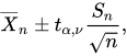
we determine that with 90% confidence we have a true mean lying below
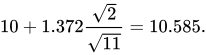
In other words, 90% of the times that an upper threshold is calculated by this method from particular samples, this upper threshold exceeds the true mean.
And with 90% confidence we have a true mean lying above
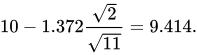
In other words, 90% of the times that a lower threshold is calculated by this method from particular samples, this lower threshold lies below the true mean.
So that at 80% confidence (calculated from 100% − 2 × (1 − 90%) = 80%), we have a true mean lying within the interval

Saying that 80% of the times that upper and lower thresholds are calculated by this method from a given sample, the true mean is both below the upper threshold and above the lower threshold is not the same as saying that there is an 80% probability that the true mean lies between a particular pair of upper and lower thresholds that have been calculated by this method; see confidence interval and prosecutor’s fallacy.
Nowadays, statistical software, such as the R programming language, and functions available in many spreadsheet programs compute values of the t-distribution and its inverse without tables.
See also[edit]
Notes[edit]
- ^ Hurst, Simon. «The Characteristic Function of the Student t Distribution». Financial Mathematics Research Report No. FMRR006-95, Statistics Research Report No. SRR044-95. Archived from the original on February 18, 2010.
- ^ Helmert FR (1875). «Über die Berechnung des wahrscheinlichen Fehlers aus einer endlichen Anzahl wahrer Beobachtungsfehler». Z. Math. U. Physik. 20: 300–3.
- ^ Helmert FR (1876). «Über die Wahrscheinlichkeit der Potenzsummen der Beobachtungsfehler und uber einige damit in Zusammenhang stehende Fragen». Z. Math. Phys. 21: 192–218.
- ^ Helmert FR (1876). «Die Genauigkeit der Formel von Peters zur Berechnung des wahrscheinlichen Beobachtungsfehlers directer Beobachtungen gleicher Genauigkeit» [The accuracy of Peters’ formula for calculating the probable observation error of direct observations of the same accuracy]. Astron. Nachr. (in German). 88 (8–9): 113–132. Bibcode:1876AN…..88..113H. doi:10.1002/asna.18760880802.
- ^ Lüroth J (1876). «Vergleichung von zwei Werten des wahrscheinlichen Fehlers». Astron. Nachr. 87 (14): 209–20. Bibcode:1876AN…..87..209L. doi:10.1002/asna.18760871402.
- ^ Pfanzagl J, Sheynin O (1996). «Studies in the history of probability and statistics. XLIV. A forerunner of the t-distribution». Biometrika. 83 (4): 891–898. doi:10.1093/biomet/83.4.891. MR 1766040.
- ^ Sheynin O (1995). «Helmert’s work in the theory of errors». Arch. Hist. Exact Sci. 49 (1): 73–104. doi:10.1007/BF00374700. S2CID 121241599.
- ^ Pearson, K. (1895-01-01). «Contributions to the Mathematical Theory of Evolution. II. Skew Variation in Homogeneous Material». Philosophical Transactions of the Royal Society A: Mathematical, Physical and Engineering Sciences. 186: 343–414 (374). Bibcode:1895RSPTA.186..343P. doi:10.1098/rsta.1895.0010. ISSN 1364-503X.
- ^ «Student» [William Sealy Gosset] (1908). «The probable error of a mean» (PDF). Biometrika. 6 (1): 1–25. doi:10.1093/biomet/6.1.1. hdl:10338.dmlcz/143545. JSTOR 2331554.
- ^ Wendl MC (2016). «Pseudonymous fame». Science. 351 (6280): 1406. Bibcode:2016Sci…351.1406W. doi:10.1126/science.351.6280.1406. PMID 27013722.
- ^ Mortimer RG (2005). Mathematics for physical chemistry (3rd ed.). Burlington, MA: Elsevier. pp. 326. ISBN 9780080492889. OCLC 156200058.
- ^ a b Fisher RA (1925). «Applications of ‘Student’s’ distribution» (PDF). Metron. 5: 90–104. Archived from the original (PDF) on 5 March 2016.
- ^ Walpole RE, Myers R, Myers S, et al. (2006). Probability & Statistics for Engineers & Scientists (7th ed.). New Delhi: Pearson. p. 237. ISBN 9788177584042. OCLC 818811849.
- ^ Kruschke JK (2015). Doing Bayesian Data Analysis (2nd ed.). Academic Press. ISBN 9780124058880. OCLC 959632184.
- ^ a b c Johnson NL, Kotz S, Balakrishnan N (1995). «Chapter 28». Continuous Univariate Distributions. Vol. 2 (2nd ed.). Wiley. ISBN 9780471584940.
- ^ Gelman AB, Carlin JS, Rubin DB, et al. (1997). Bayesian Data Analysis (2nd ed.). Boca Raton: Chapman & Hall. p. 68. ISBN 9780412039911.
- ^ Hogg RV, Craig AT (1978). Introduction to Mathematical Statistics (4th ed.). New York: Macmillan. ASIN B010WFO0SA. Sections 4.4 and 4.8
{{cite book}}: CS1 maint: postscript (link) - ^ Cochran WG (1934). «The distribution of quadratic forms in a normal system, with applications to the analysis of covariance». Math. Proc. Camb. Philos. Soc. 30 (2): 178–191. Bibcode:1934PCPS…30..178C. doi:10.1017/S0305004100016595. S2CID 122547084.
- ^ Park SY, Bera AK (2009). «Maximum entropy autoregressive conditional heteroskedasticity model». J. Econom. 150 (2): 219–230. doi:10.1016/j.jeconom.2008.12.014.
- ^ Casella G, Berger RL (1990). Statistical Inference. Duxbury Resource Center. p. 56. ISBN 9780534119584.
- ^ a b Bailey RW (1994). «Polar Generation of Random Variates with the t-Distribution». Math. Comput. 62 (206): 779–781. Bibcode:1994MaCom..62..779B. doi:10.2307/2153537. JSTOR 2153537.
- ^ a b Jackman, S. (2009). Bayesian Analysis for the Social Sciences. Wiley Series in Probability and Statistics. Wiley. p. 507. doi:10.1002/9780470686621. ISBN 9780470011546.
- ^ Platen, Eckhard & Sidorowicz, Renata (March 2007). «Empirical Evidence on Student-t Log Returns of Diversified World Stock Indices» (PDF). Quantitative Finance Research Center. ISSN 1441-8010. Archived from the original (PDF) on 2019-04-30. Retrieved 2022-03-22.
{{cite journal}}: CS1 maint: multiple names: authors list (link) - ^ a b Bishop, C.M. (2006). Pattern Recognition and Machine Learning. New York, NY: Springer. ISBN 9780387310732.
- ^ Ord JK (1972). Families of Frequency Distributions. London: Griffin. ISBN 9780852641378. See Table 5.1.
{{cite book}}: CS1 maint: postscript (link) - ^ Ord JK (1972). «Chapter 5». Families of frequency distributions. London: Griffin. ISBN 9780852641378.
- ^ Lee, Se Yoon (2022). «The Use of a Log-Normal Prior for the Student t-Distribution». Axioms. 11 (9): 462. doi:10.3390/axioms11090462.
- ^ Fonseca, T.C.; Ferreira, M.A.; Migon, H.S. (2008). «Objective Bayesian analysis for the Student-t regression model». Biometrika. 95 (2): 325–333. doi:10.1093/biomet/asn001.
- ^ Fernández, C.; Steel, M.F. (1998). «On Bayesian modeling of fat tails and skewness». J. Am. Stat. Assoc.
- ^ Juárez, M.A.; Steel, M.F. (2010). «Model-based clustering of non-Gaussian panel data based on skew-t distributions». J. Bus. Econ. Stat. 28: 52–66. doi:10.1198/jbes.2009.07145. S2CID 10091669.
- ^ Lee, Se Yoon (2022). «The Use of a Log-Normal Prior for the Student t-Distribution». Axioms. 11 (9): 462. doi:10.3390/axioms11090462.
- ^ Lange KL, Little RJ, Taylor JM (1989). «Robust Statistical Modeling Using the t Distribution» (PDF). J. Am. Stat. Assoc. 84 (408): 881–896. doi:10.1080/01621459.1989.10478852. JSTOR 2290063.
- ^ Gelman AB, Carlin JB, Stern HS, et al. (2014). «Computationally efficient Markov chain simulation». Bayesian Data Analysis. Boca Raton, Florida: CRC Press. p. 293. ISBN 9781439898208.
- ^ Shah, Amar; Wilson, Andrew Gordon; Ghahramani, Zoubin (2014). «Student-t processes as alternatives to Gaussian processes» (PDF). JMLR. 33 (Proceedings of the 17th International Conference on Artificial Intelligence and Statistics (AISTATS) 2014, Reykjavik, Iceland): 877–885. arXiv:1402.4306.
- ^ Chen, Zexun; Wang, Bo; Gorban, Alexander N. (2019). «Multivariate Gaussian and Student-t process regression for multi-output prediction». Neural Computing and Applications. 32 (8): 3005–3028. arXiv:1703.04455. doi:10.1007/s00521-019-04687-8.
- ^ Sun, Jingchao; Kong, Maiying; Pal, Subhadip (22 June 2021). «The Modified-Half-Normal distribution: Properties and an efficient sampling scheme». Communications in Statistics — Theory and Methods: 1–23. doi:10.1080/03610926.2021.1934700. ISSN 0361-0926. S2CID 237919587.
References[edit]
- Senn, S.; Richardson, W. (1994). «The first t-test». Statistics in Medicine. 13 (8): 785–803. doi:10.1002/sim.4780130802. PMID 8047737.
- Hogg RV, Craig AT (1978). Introduction to Mathematical Statistics (4th ed.). New York: Macmillan. ASIN B010WFO0SA.
- Venables, W. N.; Ripley, B. D. (2002). Modern Applied Statistics with S (Fourth ed.). Springer.
- Gelman, Andrew; John B. Carlin; Hal S. Stern; Donald B. Rubin (2003). Bayesian Data Analysis (Second ed.). CRC/Chapman & Hall. ISBN 1-58488-388-X.
External links[edit]
- «Student distribution», Encyclopedia of Mathematics, EMS Press, 2001 [1994]
- Earliest Known Uses of Some of the Words of Mathematics (S) (Remarks on the history of the term «Student’s distribution»)
- Rouaud, M. (2013), Probability, Statistics and Estimation (PDF) (short ed.) First Students on page 112.
- Student’s t-Distribution, Archived 2021-04-10 at the Wayback Machine ck12
This article is about the mathematics of Student’s t-distribution. For its uses in statistics, see Student’s t-test.
|
Probability density function
|
|
|
Cumulative distribution function
|
|
| Parameters |
degrees of freedom (real) |
|---|---|
| Support |
|
|
|
|
| CDF |
where 2F1 is the hypergeometric function |
| Mean |
0 for , otherwise undefined |
| Median | 0 |
| Mode | 0 |
| Variance |
for , ∞ for , otherwise undefined |
| Skewness |
0 for , otherwise undefined |
| Ex. kurtosis |
for , ∞ for , otherwise undefined |
| Entropy |
|
| MGF | undefined |
| CF |
|
In probability and statistics, Student’s t-distribution (or simply the t-distribution) is any member of a family of continuous probability distributions that arise when estimating the mean of a normally distributed population in situations where the sample size is small and the population’s standard deviation is unknown. It was developed by English statistician William Sealy Gosset under the pseudonym «Student».
The t-distribution plays a role in a number of widely used statistical analyses, including Student’s t-test for assessing the statistical significance of the difference between two sample means, the construction of confidence intervals for the difference between two population means, and in linear regression analysis. Student’s t-distribution also arises in the Bayesian analysis of data from a normal family.
If we take a sample of
The t-distribution is symmetric and bell-shaped, like the normal distribution. However, the t-distribution has heavier tails, meaning that it is more prone to producing values that fall far from its mean. This makes it useful for understanding the statistical behavior of certain types of ratios of random quantities, in which variation in the denominator is amplified and may produce outlying values when the denominator of the ratio falls close to zero. The Student’s t-distribution is a special case of the generalized hyperbolic distribution.
History and etymology[edit]
Statistician William Sealy Gosset, known as «Student»
In statistics, the t-distribution was first derived as a posterior distribution in 1876 by Helmert[2][3][4] and Lüroth.[5][6][7] The t-distribution also appeared in a more general form as Pearson Type IV distribution in Karl Pearson’s 1895 paper.[8]
In the English-language literature, the distribution takes its name from William Sealy Gosset’s 1908 paper in Biometrika under the pseudonym «Student».[9] One version of the origin of the pseudonym is that Gosset’s employer preferred staff to use pen names when publishing scientific papers instead of their real name, so he used the name «Student» to hide his identity. Another version is that Guinness did not want their competitors to know that they were using the t-test to determine the quality of raw material.[10][11]
Gosset worked at the Guinness Brewery in Dublin, Ireland, and was interested in the problems of small samples – for example, the chemical properties of barley where sample sizes might be as few as 3. Gosset’s paper refers to the distribution as the «frequency distribution of standard deviations of samples drawn from a normal population». It became well known through the work of Ronald Fisher, who called the distribution «Student’s distribution» and represented the test value with the letter t.[12][13]
How Student’s distribution arises from sampling[edit]
Let
Let
be the sample mean and let
be the (Bessel-corrected) sample variance. Then the random variable
has a standard normal distribution (i.e. normal with expected mean 0 and variance 1), and the random variable
i.e where
Definition[edit]
Probability density function[edit]
Student’s t-distribution has the probability density function (PDF) given by
where
where B is the Beta function. In particular for integer valued degrees of freedom
For
For
The probability density function is symmetric, and its overall shape resembles the bell shape of a normally distributed variable with mean 0 and variance 1, except that it is a bit lower and wider. As the number of degrees of freedom grows, the t-distribution approaches the normal distribution with mean 0 and variance 1. For this reason
The following images show the density of the t-distribution for increasing values of
1 degree of freedom
2 degrees of freedom
3 degrees of freedom
5 degrees of freedom
10 degrees of freedom
30 degrees of freedom
Cumulative distribution function[edit]
The cumulative distribution function (CDF) can be written in terms of I, the regularized
incomplete beta function. For t > 0,[15]
where
Other values would be obtained by symmetry. An alternative formula, valid for
where 2F1 is a particular case of the hypergeometric function.
For information on its inverse cumulative distribution function, see quantile function § Student’s t-distribution.
Special cases[edit]
Certain values of
|
|
CDF | notes | |
|---|---|---|---|
| 1 |
|
|
See Cauchy distribution |
| 2 |
|
|
|
| 3 |
|
|
|
| 4 |
|
|
|
| 5 |
|
|
|
|
|
|
|
See Normal distribution, Error function |
How the t-distribution arises[edit]
Sampling distribution[edit]
Let
The resulting t-value is
The t-distribution with
Bayesian inference[edit]
In Bayesian statistics, a (scaled, shifted) t-distribution arises as the marginal distribution of the unknown mean of a normal distribution, when the dependence on an unknown variance has been marginalized out:[16]
where
With
a normal distribution and a scaled inverse chi-squared distribution respectively, where
The marginalization integral thus becomes
This can be evaluated by substituting
so
But the z integral is now a standard Gamma integral, which evaluates to a constant, leaving
This is a form of the t-distribution with an explicit scaling and shifting that will be explored in more detail in a further section below. It can be related to the standardized t-distribution by the substitution
The derivation above has been presented for the case of uninformative priors for
Characterization[edit]
As the distribution of a test statistic[edit]
Student’s t-distribution with
where
- Z is a standard normal with expected value 0 and variance 1;
- V has a chi-squared distribution (χ2-distribution) with
- Z and V are independent;
A different distribution is defined as that of the random variable defined, for a given constant μ, by
This random variable has a noncentral t-distribution with noncentrality parameter μ. This distribution is important in studies of the power of Student’s t-test.
Derivation[edit]
Suppose X1, …, Xn are independent realizations of the normally-distributed, random variable X, which has an expected value μ and variance σ2. Let
be the sample mean, and
be an unbiased estimate of the variance from the sample. It can be shown that the random variable
has a chi-squared distribution with
is normally distributed with mean 0 and variance 1, since the sample mean
which differs from Z in that the exact standard deviation σ is replaced by the random variable Sn, has a Student’s t-distribution as defined above. Notice that the unknown population variance σ2 does not appear in T, since it was in both the numerator and the denominator, so it canceled. Gosset intuitively obtained the probability density function stated above, with
The distribution of the test statistic T depends on
As a maximum entropy distribution[edit]
Student’s t-distribution is the maximum entropy probability distribution for a random variate X for which
Properties[edit]
Moments[edit]
For
Moments of order
The term for
For a t-distribution with
Monte Carlo sampling[edit]
There are various approaches to constructing random samples from the Student’s t-distribution. The matter depends on whether the samples are required on a stand-alone basis, or are to be constructed by application of a quantile function to uniform samples; e.g., in the multi-dimensional applications basis of copula-dependency.[citation needed] In the case of stand-alone sampling, an extension of the Box–Muller method and its polar form is easily deployed.[21] It has the merit that it applies equally well to all real positive degrees of freedom, ν, while many other candidate methods fail if ν is close to zero.[21]
Integral of Student’s probability density function and p-value[edit]
The function A(t | ν) is the integral of Student’s probability density function, f(t) between −t and t, for t ≥ 0. It thus gives the probability that a value of t less than that calculated from observed data would occur by chance. Therefore, the function A(t | ν) can be used when testing whether the difference between the means of two sets of data is statistically significant, by calculating the corresponding value of t and the probability of its occurrence if the two sets of data were drawn from the same population. This is used in a variety of situations, particularly in t-tests. For the statistic t, with ν degrees of freedom, A(t | ν) is the probability that t would be less than the observed value if the two means were the same (provided that the smaller mean is subtracted from the larger, so that t ≥ 0). It can be easily calculated from the cumulative distribution function Fν(t) of the t-distribution:
where Ix is the regularized incomplete beta function (a, b).
For statistical hypothesis testing this function is used to construct the p-value.
Generalized Student’s t-distribution[edit]
In terms of scaling parameter σ̂ or σ̂2[edit]
Student’s t distribution can be generalized to a three parameter location-scale family, introducing a location parameter
or
This means that
The resulting non-standardized Student’s t-distribution has a density defined by:[22]
Here,
Equivalently, the distribution can be written in terms of
Other properties of this version of the distribution are:[22]
This distribution results from compounding a Gaussian distribution (normal distribution) with mean
Equivalently, this distribution results from compounding a Gaussian distribution with a scaled-inverse-chi-squared distribution with parameters
This version of the t-distribution can be useful in financial modeling. For example, Platen and Sidorowicz found that among the family of generalized hyperbolic distributions, this form of the t-distribution with about 4 degrees of freedom was the best fit for the (log) return of many worldwide stock indices.[23]
In terms of inverse scaling parameter λ[edit]
An alternative parameterization in terms of an inverse scaling parameter
Other properties of this version of the distribution are:[24]
This distribution results from compounding a Gaussian distribution with mean
[edit]
- If
- The noncentral t-distribution generalizes the t-distribution to include a location parameter. Unlike the nonstandardized t-distributions, the noncentral distributions are not symmetric (the median is not the same as the mode).
- The discrete Student’s t-distribution is defined by its probability mass function at r being proportional to:[25]
Here a, b, and k are parameters. This distribution arises from the construction of a system of discrete distributions similar to that of the Pearson distributions for continuous distributions.[26]
- One can generate Student-t samples by taking the ratio of variables from the normal distribution and the square-root of χ2-distribution. If we use instead of the normal distribution, e.g., the Irwin–Hall distribution, we obtain over-all a symmetric 4-parameter distribution, which includes the normal, the uniform, the triangular, the Student-t and the Cauchy distribution. This is also more flexible than some other symmetric generalizations of the normal distribution.
- t-distribution is an instance of ratio distributions.
Bayesian inference: prior distribution for the degrees of the freedom[edit]
Suppose that
With a choice a prior for the degrees of freedom
Mean squared error comparison between Bayes estimators based on the four priors and maximum likelihood estimator for the degrees of the freedom. Data is simulated from the student t distribution with the degrees of freedom
Some popular choices of the priors are:
- Jeffreys prior [28]
where
- Exponential prior [29]
- Gamma prior [30]
- Log-normal prior [31]
The right panels show the result of the numerical experiments. The Bayes estimator based on the Jeffreys prior
Uses[edit]
In frequentist statistical inference[edit]
Student’s t-distribution arises in a variety of statistical estimation problems where the goal is to estimate an unknown parameter, such as a mean value, in a setting where the data are observed with additive errors. If (as in nearly all practical statistical work) the population standard deviation of these errors is unknown and has to be estimated from the data, the t-distribution is often used to account for the extra uncertainty that results from this estimation. In most such problems, if the standard deviation of the errors were known, a normal distribution would be used instead of the t-distribution.
Confidence intervals and hypothesis tests are two statistical procedures in which the quantiles of the sampling distribution of a particular statistic (e.g. the standard score) are required. In any situation where this statistic is a linear function of the data, divided by the usual estimate of the standard deviation, the resulting quantity can be rescaled and centered to follow Student’s t-distribution. Statistical analyses involving means, weighted means, and regression coefficients all lead to statistics having this form.
Quite often, textbook problems will treat the population standard deviation as if it were known and thereby avoid the need to use the Student’s t-distribution. These problems are generally of two kinds: (1) those in which the sample size is so large that one may treat a data-based estimate of the variance as if it were certain, and (2) those that illustrate mathematical reasoning, in which the problem of estimating the standard deviation is temporarily ignored because that is not the point that the author or instructor is then explaining.
Hypothesis testing[edit]
A number of statistics can be shown to have t-distributions for samples of moderate size under null hypotheses that are of interest, so that the t-distribution forms the basis for significance tests. For example, the distribution of Spearman’s rank correlation coefficient ρ, in the null case (zero correlation) is well approximated by the t distribution for sample sizes above about 20.[citation needed]
Confidence intervals[edit]
Suppose the number A is so chosen that
when T has a t-distribution with n − 1 degrees of freedom. By symmetry, this is the same as saying that A satisfies
so A is the «95th percentile» of this probability distribution, or
and this is equivalent to
Therefore, the interval whose endpoints are
is a 90% confidence interval for μ. Therefore, if we find the mean of a set of observations that we can reasonably expect to have a normal distribution, we can use the t-distribution to examine whether the confidence limits on that mean include some theoretically predicted value – such as the value predicted on a null hypothesis.
It is this result that is used in the Student’s t-tests: since the difference between the means of samples from two normal distributions is itself distributed normally, the t-distribution can be used to examine whether that difference can reasonably be supposed to be zero.
If the data are normally distributed, the one-sided (1 − α)-upper confidence limit (UCL) of the mean, can be calculated using the following equation:
The resulting UCL will be the greatest average value that will occur for a given confidence interval and population size. In other words,
Prediction intervals[edit]
The t-distribution can be used to construct a prediction interval for an unobserved sample from a normal distribution with unknown mean and variance.
In Bayesian statistics[edit]
The Student’s t-distribution, especially in its three-parameter (location-scale) version, arises frequently in Bayesian statistics as a result of its connection with the normal distribution. Whenever the variance of a normally distributed random variable is unknown and a conjugate prior placed over it that follows an inverse gamma distribution, the resulting marginal distribution of the variable will follow a Student’s t-distribution. Equivalent constructions with the same results involve a conjugate scaled-inverse-chi-squared distribution over the variance, or a conjugate gamma distribution over the precision. If an improper prior proportional to σ−2 is placed over the variance, the t-distribution also arises. This is the case regardless of whether the mean of the normally distributed variable is known, is unknown distributed according to a conjugate normally distributed prior, or is unknown distributed according to an improper constant prior.
Related situations that also produce a t-distribution are:
- The marginal posterior distribution of the unknown mean of a normally distributed variable, with unknown prior mean and variance following the above model.
- The prior predictive distribution and posterior predictive distribution of a new normally distributed data point when a series of independent identically distributed normally distributed data points have been observed, with prior mean and variance as in the above model.
Robust parametric modeling[edit]
The t-distribution is often used as an alternative to the normal distribution as a model for data, which often has heavier tails than the normal distribution allows for; see e.g. Lange et al.[32] The classical approach was to identify outliers (e.g., using Grubbs’s test) and exclude or downweight them in some way. However, it is not always easy to identify outliers (especially in high dimensions), and the t-distribution is a natural choice of model for such data and provides a parametric approach to robust statistics.
A Bayesian account can be found in Gelman et al.[33] The degrees of freedom parameter controls the kurtosis of the distribution and is correlated with the scale parameter. The likelihood can have multiple local maxima and, as such, it is often necessary to fix the degrees of freedom at a fairly low value and estimate the other parameters taking this as given. Some authors[citation needed] report that values between 3 and 9 are often good choices. Venables and Ripley[citation needed] suggest that a value of 5 is often a good choice.
Student’s t-process[edit]
For practical regression and prediction needs, Student’s t-processes were introduced, that are generalisations of the Student t-distributions for functions. A Student’s t-process is constructed from the Student t-distributions like a Gaussian process is constructed from the Gaussian distributions. For a Gaussian process, all sets of values have a multidimensional Gaussian distribution. Analogously,
Table of selected values[edit]
The following table lists values for t-distributions with ν degrees of freedom for a range of one-sided or two-sided critical regions. The first column is ν, the percentages along the top are confidence levels, and the numbers in the body of the table are the
The last row with infinite ν gives critical points for a normal distribution since a t-distribution with infinitely many degrees of freedom is a normal distribution. (See Related distributions above).
| One-sided | 75% | 80% | 85% | 90% | 95% | 97.5% | 99% | 99.5% | 99.75% | 99.9% | 99.95% |
|---|---|---|---|---|---|---|---|---|---|---|---|
| Two-sided | 50% | 60% | 70% | 80% | 90% | 95% | 98% | 99% | 99.5% | 99.8% | 99.9% |
| 1 | 1.000 | 1.376 | 1.963 | 3.078 | 6.314 | 12.706 | 31.821 | 63.657 | 127.321 | 318.309 | 636.619 |
| 2 | 0.816 | 1.080 | 1.386 | 1.886 | 2.920 | 4.303 | 6.965 | 9.925 | 14.089 | 22.327 | 31.599 |
| 3 | 0.765 | 0.978 | 1.250 | 1.638 | 2.353 | 3.182 | 4.541 | 5.841 | 7.453 | 10.215 | 12.924 |
| 4 | 0.741 | 0.941 | 1.190 | 1.533 | 2.132 | 2.776 | 3.747 | 4.604 | 5.598 | 7.173 | 8.610 |
| 5 | 0.727 | 0.920 | 1.156 | 1.476 | 2.015 | 2.571 | 3.365 | 4.032 | 4.773 | 5.893 | 6.869 |
| 6 | 0.718 | 0.906 | 1.134 | 1.440 | 1.943 | 2.447 | 3.143 | 3.707 | 4.317 | 5.208 | 5.959 |
| 7 | 0.711 | 0.896 | 1.119 | 1.415 | 1.895 | 2.365 | 2.998 | 3.499 | 4.029 | 4.785 | 5.408 |
| 8 | 0.706 | 0.889 | 1.108 | 1.397 | 1.860 | 2.306 | 2.896 | 3.355 | 3.833 | 4.501 | 5.041 |
| 9 | 0.703 | 0.883 | 1.100 | 1.383 | 1.833 | 2.262 | 2.821 | 3.250 | 3.690 | 4.297 | 4.781 |
| 10 | 0.700 | 0.879 | 1.093 | 1.372 | 1.812 | 2.228 | 2.764 | 3.169 | 3.581 | 4.144 | 4.587 |
| 11 | 0.697 | 0.876 | 1.088 | 1.363 | 1.796 | 2.201 | 2.718 | 3.106 | 3.497 | 4.025 | 4.437 |
| 12 | 0.695 | 0.873 | 1.083 | 1.356 | 1.782 | 2.179 | 2.681 | 3.055 | 3.428 | 3.930 | 4.318 |
| 13 | 0.694 | 0.870 | 1.079 | 1.350 | 1.771 | 2.160 | 2.650 | 3.012 | 3.372 | 3.852 | 4.221 |
| 14 | 0.692 | 0.868 | 1.076 | 1.345 | 1.761 | 2.145 | 2.624 | 2.977 | 3.326 | 3.787 | 4.140 |
| 15 | 0.691 | 0.866 | 1.074 | 1.341 | 1.753 | 2.131 | 2.602 | 2.947 | 3.286 | 3.733 | 4.073 |
| 16 | 0.690 | 0.865 | 1.071 | 1.337 | 1.746 | 2.120 | 2.583 | 2.921 | 3.252 | 3.686 | 4.015 |
| 17 | 0.689 | 0.863 | 1.069 | 1.333 | 1.740 | 2.110 | 2.567 | 2.898 | 3.222 | 3.646 | 3.965 |
| 18 | 0.688 | 0.862 | 1.067 | 1.330 | 1.734 | 2.101 | 2.552 | 2.878 | 3.197 | 3.610 | 3.922 |
| 19 | 0.688 | 0.861 | 1.066 | 1.328 | 1.729 | 2.093 | 2.539 | 2.861 | 3.174 | 3.579 | 3.883 |
| 20 | 0.687 | 0.860 | 1.064 | 1.325 | 1.725 | 2.086 | 2.528 | 2.845 | 3.153 | 3.552 | 3.850 |
| 21 | 0.686 | 0.859 | 1.063 | 1.323 | 1.721 | 2.080 | 2.518 | 2.831 | 3.135 | 3.527 | 3.819 |
| 22 | 0.686 | 0.858 | 1.061 | 1.321 | 1.717 | 2.074 | 2.508 | 2.819 | 3.119 | 3.505 | 3.792 |
| 23 | 0.685 | 0.858 | 1.060 | 1.319 | 1.714 | 2.069 | 2.500 | 2.807 | 3.104 | 3.485 | 3.767 |
| 24 | 0.685 | 0.857 | 1.059 | 1.318 | 1.711 | 2.064 | 2.492 | 2.797 | 3.091 | 3.467 | 3.745 |
| 25 | 0.684 | 0.856 | 1.058 | 1.316 | 1.708 | 2.060 | 2.485 | 2.787 | 3.078 | 3.450 | 3.725 |
| 26 | 0.684 | 0.856 | 1.058 | 1.315 | 1.706 | 2.056 | 2.479 | 2.779 | 3.067 | 3.435 | 3.707 |
| 27 | 0.684 | 0.855 | 1.057 | 1.314 | 1.703 | 2.052 | 2.473 | 2.771 | 3.057 | 3.421 | 3.690 |
| 28 | 0.683 | 0.855 | 1.056 | 1.313 | 1.701 | 2.048 | 2.467 | 2.763 | 3.047 | 3.408 | 3.674 |
| 29 | 0.683 | 0.854 | 1.055 | 1.311 | 1.699 | 2.045 | 2.462 | 2.756 | 3.038 | 3.396 | 3.659 |
| 30 | 0.683 | 0.854 | 1.055 | 1.310 | 1.697 | 2.042 | 2.457 | 2.750 | 3.030 | 3.385 | 3.646 |
| 40 | 0.681 | 0.851 | 1.050 | 1.303 | 1.684 | 2.021 | 2.423 | 2.704 | 2.971 | 3.307 | 3.551 |
| 50 | 0.679 | 0.849 | 1.047 | 1.299 | 1.676 | 2.009 | 2.403 | 2.678 | 2.937 | 3.261 | 3.496 |
| 60 | 0.679 | 0.848 | 1.045 | 1.296 | 1.671 | 2.000 | 2.390 | 2.660 | 2.915 | 3.232 | 3.460 |
| 80 | 0.678 | 0.846 | 1.043 | 1.292 | 1.664 | 1.990 | 2.374 | 2.639 | 2.887 | 3.195 | 3.416 |
| 100 | 0.677 | 0.845 | 1.042 | 1.290 | 1.660 | 1.984 | 2.364 | 2.626 | 2.871 | 3.174 | 3.390 |
| 120 | 0.677 | 0.845 | 1.041 | 1.289 | 1.658 | 1.980 | 2.358 | 2.617 | 2.860 | 3.160 | 3.373 |
| ∞ | 0.674 | 0.842 | 1.036 | 1.282 | 1.645 | 1.960 | 2.326 | 2.576 | 2.807 | 3.090 | 3.291 |
| One-sided | 75% | 80% | 85% | 90% | 95% | 97.5% | 99% | 99.5% | 99.75% | 99.9% | 99.95% |
| Two-sided | 50% | 60% | 70% | 80% | 90% | 95% | 98% | 99% | 99.5% | 99.8% | 99.9% |
Calculating the confidence interval
Let’s say we have a sample with size 11, sample mean 10, and sample variance 2. For 90% confidence with 10 degrees of freedom, the one-sided t-value from the table is 1.372. Then with confidence interval calculated from
we determine that with 90% confidence we have a true mean lying below
In other words, 90% of the times that an upper threshold is calculated by this method from particular samples, this upper threshold exceeds the true mean.
And with 90% confidence we have a true mean lying above
In other words, 90% of the times that a lower threshold is calculated by this method from particular samples, this lower threshold lies below the true mean.
So that at 80% confidence (calculated from 100% − 2 × (1 − 90%) = 80%), we have a true mean lying within the interval
Saying that 80% of the times that upper and lower thresholds are calculated by this method from a given sample, the true mean is both below the upper threshold and above the lower threshold is not the same as saying that there is an 80% probability that the true mean lies between a particular pair of upper and lower thresholds that have been calculated by this method; see confidence interval and prosecutor’s fallacy.
Nowadays, statistical software, such as the R programming language, and functions available in many spreadsheet programs compute values of the t-distribution and its inverse without tables.
See also[edit]
Notes[edit]
- ^ Hurst, Simon. «The Characteristic Function of the Student t Distribution». Financial Mathematics Research Report No. FMRR006-95, Statistics Research Report No. SRR044-95. Archived from the original on February 18, 2010.
- ^ Helmert FR (1875). «Über die Berechnung des wahrscheinlichen Fehlers aus einer endlichen Anzahl wahrer Beobachtungsfehler». Z. Math. U. Physik. 20: 300–3.
- ^ Helmert FR (1876). «Über die Wahrscheinlichkeit der Potenzsummen der Beobachtungsfehler und uber einige damit in Zusammenhang stehende Fragen». Z. Math. Phys. 21: 192–218.
- ^ Helmert FR (1876). «Die Genauigkeit der Formel von Peters zur Berechnung des wahrscheinlichen Beobachtungsfehlers directer Beobachtungen gleicher Genauigkeit» [The accuracy of Peters’ formula for calculating the probable observation error of direct observations of the same accuracy]. Astron. Nachr. (in German). 88 (8–9): 113–132. Bibcode:1876AN…..88..113H. doi:10.1002/asna.18760880802.
- ^ Lüroth J (1876). «Vergleichung von zwei Werten des wahrscheinlichen Fehlers». Astron. Nachr. 87 (14): 209–20. Bibcode:1876AN…..87..209L. doi:10.1002/asna.18760871402.
- ^ Pfanzagl J, Sheynin O (1996). «Studies in the history of probability and statistics. XLIV. A forerunner of the t-distribution». Biometrika. 83 (4): 891–898. doi:10.1093/biomet/83.4.891. MR 1766040.
- ^ Sheynin O (1995). «Helmert’s work in the theory of errors». Arch. Hist. Exact Sci. 49 (1): 73–104. doi:10.1007/BF00374700. S2CID 121241599.
- ^ Pearson, K. (1895-01-01). «Contributions to the Mathematical Theory of Evolution. II. Skew Variation in Homogeneous Material». Philosophical Transactions of the Royal Society A: Mathematical, Physical and Engineering Sciences. 186: 343–414 (374). Bibcode:1895RSPTA.186..343P. doi:10.1098/rsta.1895.0010. ISSN 1364-503X.
- ^ «Student» [William Sealy Gosset] (1908). «The probable error of a mean» (PDF). Biometrika. 6 (1): 1–25. doi:10.1093/biomet/6.1.1. hdl:10338.dmlcz/143545. JSTOR 2331554.
- ^ Wendl MC (2016). «Pseudonymous fame». Science. 351 (6280): 1406. Bibcode:2016Sci…351.1406W. doi:10.1126/science.351.6280.1406. PMID 27013722.
- ^ Mortimer RG (2005). Mathematics for physical chemistry (3rd ed.). Burlington, MA: Elsevier. pp. 326. ISBN 9780080492889. OCLC 156200058.
- ^ a b Fisher RA (1925). «Applications of ‘Student’s’ distribution» (PDF). Metron. 5: 90–104. Archived from the original (PDF) on 5 March 2016.
- ^ Walpole RE, Myers R, Myers S, et al. (2006). Probability & Statistics for Engineers & Scientists (7th ed.). New Delhi: Pearson. p. 237. ISBN 9788177584042. OCLC 818811849.
- ^ Kruschke JK (2015). Doing Bayesian Data Analysis (2nd ed.). Academic Press. ISBN 9780124058880. OCLC 959632184.
- ^ a b c Johnson NL, Kotz S, Balakrishnan N (1995). «Chapter 28». Continuous Univariate Distributions. Vol. 2 (2nd ed.). Wiley. ISBN 9780471584940.
- ^ Gelman AB, Carlin JS, Rubin DB, et al. (1997). Bayesian Data Analysis (2nd ed.). Boca Raton: Chapman & Hall. p. 68. ISBN 9780412039911.
- ^ Hogg RV, Craig AT (1978). Introduction to Mathematical Statistics (4th ed.). New York: Macmillan. ASIN B010WFO0SA. Sections 4.4 and 4.8
{{cite book}}: CS1 maint: postscript (link) - ^ Cochran WG (1934). «The distribution of quadratic forms in a normal system, with applications to the analysis of covariance». Math. Proc. Camb. Philos. Soc. 30 (2): 178–191. Bibcode:1934PCPS…30..178C. doi:10.1017/S0305004100016595. S2CID 122547084.
- ^ Park SY, Bera AK (2009). «Maximum entropy autoregressive conditional heteroskedasticity model». J. Econom. 150 (2): 219–230. doi:10.1016/j.jeconom.2008.12.014.
- ^ Casella G, Berger RL (1990). Statistical Inference. Duxbury Resource Center. p. 56. ISBN 9780534119584.
- ^ a b Bailey RW (1994). «Polar Generation of Random Variates with the t-Distribution». Math. Comput. 62 (206): 779–781. Bibcode:1994MaCom..62..779B. doi:10.2307/2153537. JSTOR 2153537.
- ^ a b Jackman, S. (2009). Bayesian Analysis for the Social Sciences. Wiley Series in Probability and Statistics. Wiley. p. 507. doi:10.1002/9780470686621. ISBN 9780470011546.
- ^ Platen, Eckhard & Sidorowicz, Renata (March 2007). «Empirical Evidence on Student-t Log Returns of Diversified World Stock Indices» (PDF). Quantitative Finance Research Center. ISSN 1441-8010. Archived from the original (PDF) on 2019-04-30. Retrieved 2022-03-22.
{{cite journal}}: CS1 maint: multiple names: authors list (link) - ^ a b Bishop, C.M. (2006). Pattern Recognition and Machine Learning. New York, NY: Springer. ISBN 9780387310732.
- ^ Ord JK (1972). Families of Frequency Distributions. London: Griffin. ISBN 9780852641378. See Table 5.1.
{{cite book}}: CS1 maint: postscript (link) - ^ Ord JK (1972). «Chapter 5». Families of frequency distributions. London: Griffin. ISBN 9780852641378.
- ^ Lee, Se Yoon (2022). «The Use of a Log-Normal Prior for the Student t-Distribution». Axioms. 11 (9): 462. doi:10.3390/axioms11090462.
- ^ Fonseca, T.C.; Ferreira, M.A.; Migon, H.S. (2008). «Objective Bayesian analysis for the Student-t regression model». Biometrika. 95 (2): 325–333. doi:10.1093/biomet/asn001.
- ^ Fernández, C.; Steel, M.F. (1998). «On Bayesian modeling of fat tails and skewness». J. Am. Stat. Assoc.
- ^ Juárez, M.A.; Steel, M.F. (2010). «Model-based clustering of non-Gaussian panel data based on skew-t distributions». J. Bus. Econ. Stat. 28: 52–66. doi:10.1198/jbes.2009.07145. S2CID 10091669.
- ^ Lee, Se Yoon (2022). «The Use of a Log-Normal Prior for the Student t-Distribution». Axioms. 11 (9): 462. doi:10.3390/axioms11090462.
- ^ Lange KL, Little RJ, Taylor JM (1989). «Robust Statistical Modeling Using the t Distribution» (PDF). J. Am. Stat. Assoc. 84 (408): 881–896. doi:10.1080/01621459.1989.10478852. JSTOR 2290063.
- ^ Gelman AB, Carlin JB, Stern HS, et al. (2014). «Computationally efficient Markov chain simulation». Bayesian Data Analysis. Boca Raton, Florida: CRC Press. p. 293. ISBN 9781439898208.
- ^ Shah, Amar; Wilson, Andrew Gordon; Ghahramani, Zoubin (2014). «Student-t processes as alternatives to Gaussian processes» (PDF). JMLR. 33 (Proceedings of the 17th International Conference on Artificial Intelligence and Statistics (AISTATS) 2014, Reykjavik, Iceland): 877–885. arXiv:1402.4306.
- ^ Chen, Zexun; Wang, Bo; Gorban, Alexander N. (2019). «Multivariate Gaussian and Student-t process regression for multi-output prediction». Neural Computing and Applications. 32 (8): 3005–3028. arXiv:1703.04455. doi:10.1007/s00521-019-04687-8.
- ^ Sun, Jingchao; Kong, Maiying; Pal, Subhadip (22 June 2021). «The Modified-Half-Normal distribution: Properties and an efficient sampling scheme». Communications in Statistics — Theory and Methods: 1–23. doi:10.1080/03610926.2021.1934700. ISSN 0361-0926. S2CID 237919587.
References[edit]
- Senn, S.; Richardson, W. (1994). «The first t-test». Statistics in Medicine. 13 (8): 785–803. doi:10.1002/sim.4780130802. PMID 8047737.
- Hogg RV, Craig AT (1978). Introduction to Mathematical Statistics (4th ed.). New York: Macmillan. ASIN B010WFO0SA.
- Venables, W. N.; Ripley, B. D. (2002). Modern Applied Statistics with S (Fourth ed.). Springer.
- Gelman, Andrew; John B. Carlin; Hal S. Stern; Donald B. Rubin (2003). Bayesian Data Analysis (Second ed.). CRC/Chapman & Hall. ISBN 1-58488-388-X.
External links[edit]
- «Student distribution», Encyclopedia of Mathematics, EMS Press, 2001 [1994]
- Earliest Known Uses of Some of the Words of Mathematics (S) (Remarks on the history of the term «Student’s distribution»)
- Rouaud, M. (2013), Probability, Statistics and Estimation (PDF) (short ed.) First Students on page 112.
- Student’s t-Distribution, Archived 2021-04-10 at the Wayback Machine ck12