Power query функция если ошибка

In Excel we can use IFERROR to if our calculation results in an error, and we can then tell Excel to produce a different result, instead of the error.

Power Query doesn’t have IFERROR but it does have a way of checking for errors and replacing that error with a default answer, it’s called try otherwise

In this post I’ll show you how to use try otherwise to handle errors when loading data, how to handle errors in your transformations and how to handle errors when your query can’t locate a data source.

Download Sample Excel Workbook

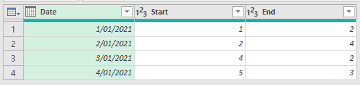
First up, let’s load data from this table.

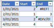
I’ve already generated a couple of errors in this table, and of course I can obviously see them and I could fix them before loading into Power Query.

But when using Power Query this isn’t always the situation. Your query will be loading data without knowing what it is so how would it handle these errors?

Let’s load the data into Power Query and call it Errors from Sheet

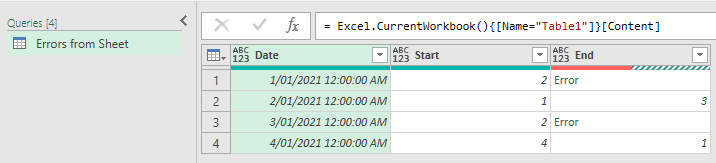
Straight away you can see the errors in the column.

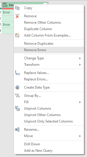
Now of course you could use Remove Errors but that would remove the rows with the errors and that’s not what I want.

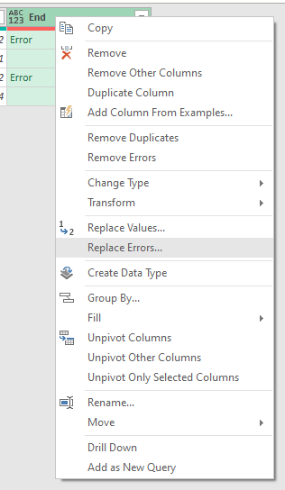
Or I could use Replace Errors, but this doesn’t give me any idea what the cause of the error is.

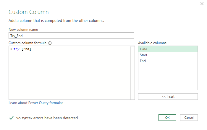
I want to see what caused the error and to do this I’ll add a Custom Column and use try [End]

This creates a new column with a Record in each row

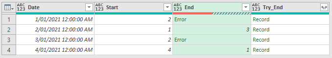
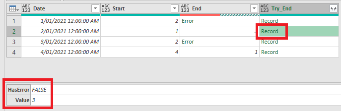
In this record are two fields. HasError states whether or not there’s an error in the [End] column

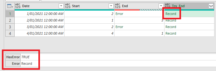
If there is an Error then the 2nd field is another record containing information about that error

If there isn’t an error, then the 2nd field is the value from the [End] column

If I expand the new column I get 3 new columns containing the HasError value which is boolean, and either an Error or a Value

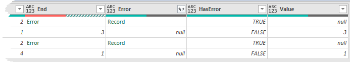
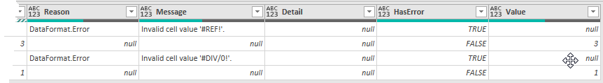
Checking what’s in the Error Records, you can see the Reason for the error, DataFormat.Error, this is from Power Query

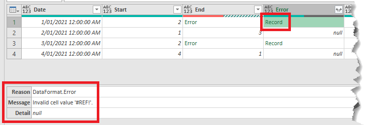
There’s the Message, which is the error from the Excel sheet, and some errors give extra Detail, but not in this case.

If I expand this Error column I can see all of these fields.

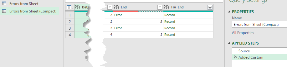
I’ve ended up with a lot of extra columns here and it’s a bit messy so let’s tidy it up. In fact I’ll duplicate the query and show you another way to get the same information in a neater way

The new query is called Errors from Sheet (Compact) and I’ve deleted all steps except the first two.

What I want to do is , check for an error in the Try_End column, and if there is one I want to see the error message from Excel.

If there isn’t an error I want the value from the [End] column.

I can do all of this in a new column using an if then else

Add a new Custom Column called Error or Value and enter this code

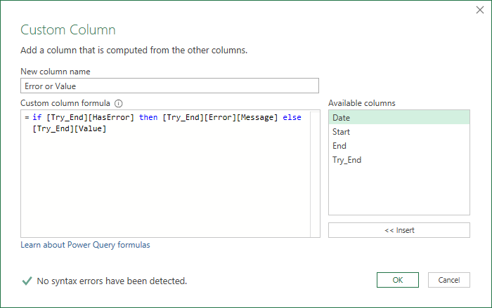
What this is saying is:

• If the boolean value [HasError] in the [Try_End] column is true then
• return the [Message] in the [Error] record of the [Try_End] column
• else return the [Value] from the [Try_End] column

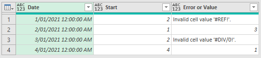
With that written I can remove both the End and Try_End columns so the final table looks like this

Checking for Errors and Replacing Them With Default Values

In this scenario I don’t care what the error is or what caused it, I just want to make sure my calculations don’t fail.

I duplicate the original query again, calling this one Error in Calculation, and remove every step except the Source step

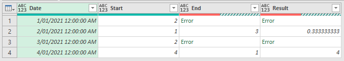
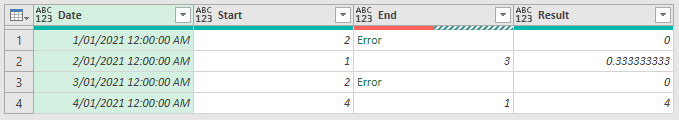
I add a new Custom column called Result and what I’ll do here is divide [Start] by [End]

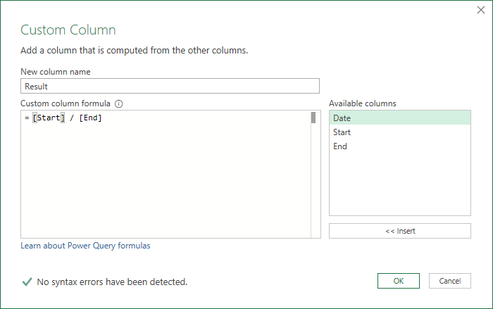
this gives me an error as I know it will in rows 1 and 3

so to avoid this, edit the step and use try .. otherwise

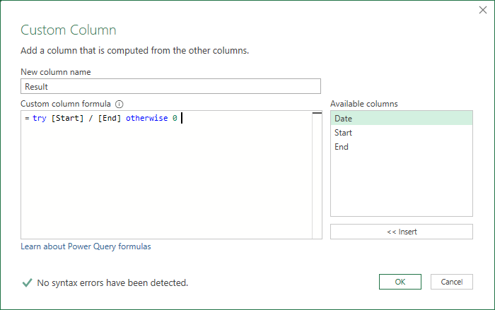
now the errors are replaced with 0.

Errors Loading Data from A Data Source

I’ll create a new query and load from an Excel workbook

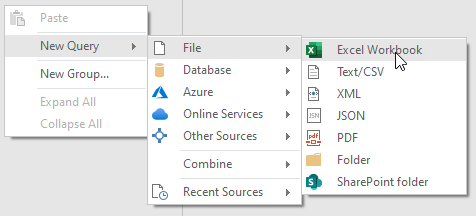
Navigating to the file I want I load it

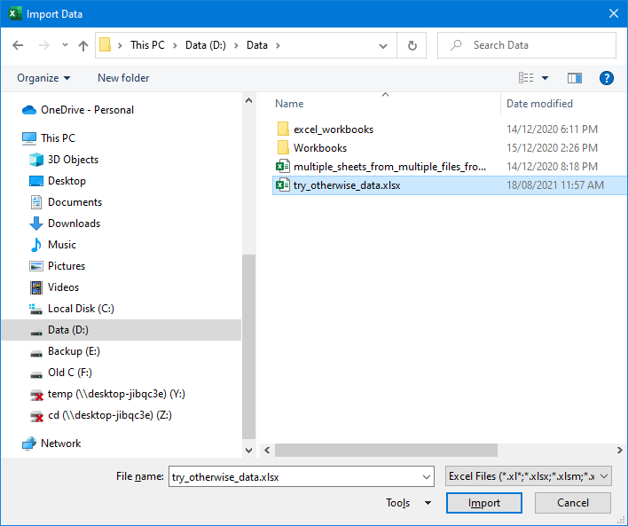
and loading this table

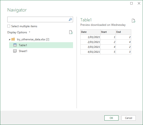
I’m not going to do any transformations because I just want to show you how to deal with errors finding this source file.

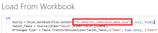
I’ll open the Advanced Editor (Home -> Advanced Editor) and change the path, so that I know I’ll get an error. Here I change the drive letter to X.

I don’t have an X: drive so I know this will cause the workbook loading to fail.

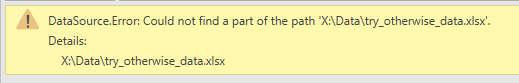
So that’s what happens when the file can’t be found so let’s say I have a backup or alternate file that I want to load if my main file can’t be found.

Open the Advanced Editor again and then use try otherwise to specify the backup file’s location

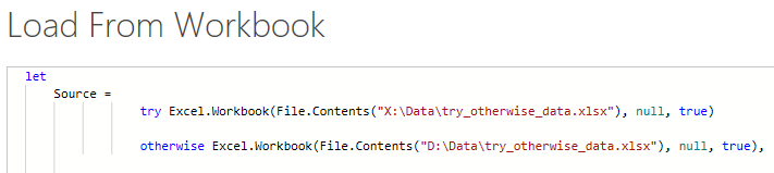
close the editor and now my backup file is loaded.

IMPORTANT: You can read the official documentation that Microsoft has on this topic from the following link (url).

If you haven’t read the first two posts (Part 1 | Part 2) in this series yet, I welcome you to do so before reading this one.

I also recommend that you check out this post on Query Error Auditing so you get a better understanding of what types of errors you can find in Power BI / Power Query.

This is a post on how to use error handling, similar to an IFERROR in DAX and Excel, but for Power Query (using its M language).

How does Error handling works in Excel & DAX?

In Excel and in DAX we have the IFERROR function which works like this:

=IFERROR( value, value_if_error)

Taken directly from the official DAX documentation:

Evaluates an expression and returns a specified value if the expression returns an error; otherwise returns the value of the expression itself.

It’s a pretty simple and straightforward function in DAX and Excel, where you can enter your formula in the “value” parameter and then, if you get an error from it, you can define what should be the output value in the “value_if_error” parameter.

The whole idea is that you can “catch” an error and use a different value when it finds an error.

How does Error handling works in Power BI / Power Query?

In Power Query the code is a bit different. Let’s see it in action and then talk more about it.

Imagine that we have an Excel workbook with a table like this

:

What we would like to create is a new column that should multiply the values from the [Price] and [Amount] columns to create a new Subtotal column.

One caveat, as you can probably see, is that this spreadsheet has some cells with errors on the [Price] column. In the event that we find an error on the Price column, we need to use the value from the [List Price] instead of the [Price] value.

The first thing that we need to do is import that table from Excel. If you’d like to follow along, you can download the workbook by clicking the button below:

Importing data from the Excel Workbook

I’ll be using Power BI Desktop for this, but you can use Excel as well.

The first thing that we need to do is select the Excel connector and connect to our file:

and once you get the “Navigator” window, you can select the table that reads “Sample”:

Notice how there’s a bunch of errors in that [Price] column just in the preview. Let’s hit the “Edit” button so we can go to the Power Query Editor Window.

Using error handling in Power BI /Power Query

Now that we have our data in the Power Query Editor window:

what we want to do is create a Custom Column, so we simply go to the “Add Column” menu and hit on “Custom Column”.

In there, we try do create a simple column that will multiply the [Price] column by the [Amount] column:

and as you can see, our [Subtotal] column has some errors.

We know that in Excel and DAX you can use IFERROR, but what can you use in Power Query ?

For Power Query, we need to hit modify that Custom Column code (just click the gear icon next to the Added Custom step) and add the following pieces to it:

try [Price]*[Amount] otherwise [Amount]*[List Price]

We need to use the keywords “try” and “otherwise”. It’s pretty easy to read, but it just says to try and evaluate the expression ([Price] * [Amount]) and if that gives an error, use the expression defined after the otherwise statement.

The result of that will look like this:

pretty simple! almost as simple as the IFERROR function in DAX and Excel where intellisense does explain you a bit how to use that function, but in Power Query you need to understand how this works in order to use it. Is nowhere in the User Interface of Power Query, so you need to write this code manually.

Understanding Errors

The workbook sample that I’m using is fairly simple. I’ve had experiences where some users / customers absolutely need to know when a specific error is found from an Excel Workbook.

What happens with Power Query is that it just flags any errors found as “Error” but, what if you needed to know WHY it shows as an error?

Let’s go back to our initial load of the file. Remember that in most cases Power Query will automatically try to add a “Changed Type” step, so what if we remove that step?

Well, I removed the step and I’m still seeing the errors and that’s because the error wasn’t triggered by a data type conversion, but rather it’s a source error, meaning that the error comes directly from the Excel Workbook.

In Workbook with vast amounts of rows, it’s hard to tell if there are any errors at all and doing a “Replace Errors” will not tell us why those errors occurred. We NEED to know what is the error from the source because we want to handle each type of error differently.

Error Message and Error Reason

To figure out what’s the reason why there’s an error, we need to use the “try” statement again.

Note how I only use “try” and not the “otherwise” statement. This will give me a new column with record values. We can expand those records like this:

the most important field from those records it’s the “Error” field which can be either a null or a record value:

and after expanding that column and deleting some others that we don’t need, I end up with this:

I’ve highlighted the most important field after this whole process which is the “Message” which tells me exactly the reason why this is an error.

I can later use this to my advantage and target specific errors differently or get a report of ALL the errors found on a series of files that my department / group uses. This is extremely helpful if you’re trying to validate everything and make sure that we don’t have any errors at the source.

Don’t forget that these same principles work for both Step and cell Value level errors.

В Excel Power Query оператор IF — одна из самых популярных функций для проверки условия и возврата определенного значения в зависимости от того, является ли результат ИСТИНА или ЛОЖЬ. Между этим оператором if и функцией ЕСЛИ в Excel есть некоторые различия. В этом уроке я познакомлю вас с синтаксисом этого оператора if и несколькими простыми и сложными примерами.

Базовый синтаксис оператора if в Power Query

Оператор Power Query if с использованием условного столбца

• Пример 1. Базовый оператор if
• Пример 2. Сложный оператор if

Power Query if, написав M-код

• Пример 1. Базовый оператор if
• Пример 2. Сложный оператор if
  • Вложенные операторы if
  • Оператор if с логикой ИЛИ
  • Оператор if с логикой AND
  • Если оператор с логиками ИЛИ и И

Базовый синтаксис оператора if в Power Query

В Power Query синтаксис такой:

= если логическая_проверка, то значение_если_истина, иначе значение_если_ложь

• логический_тест: условие, которое вы хотите проверить.
• значение_если_истина: возвращаемое значение, если результат TRUE.
• значение_если_ложь: возвращаемое значение, если результат FALSE.

Внимание: оператор Power Query if чувствителен к регистру, если, то и еще должны быть строчными.

В Excel Power Query существует два способа создания условной логики такого типа:

• Использование функции условного столбца для некоторых основных сценариев;
• Написание M-кода для более сложных сценариев.

В следующем разделе я расскажу о некоторых примерах использования этого оператора if.

Оператор Power Query if с использованием условного столбца

 Пример 1. Базовый оператор if

Здесь я расскажу, как использовать этот оператор if в Power Query. Например, у меня есть следующий отчет о продукте, если статус продукта «Старый», отображается скидка 50%; если статус продукта «Новый», отображается скидка 20%, как показано ниже.

1. Выберите таблицу данных на листе, затем в Excel 2019 и Excel 365 щелкните Данные > Из таблицы/диапазона, см. снимок экрана:

Внимание: в Excel 2016 и Excel 2021 нажмите Данные > Из таблицы, см. снимок экрана:

2. Затем в открытом Редактор Power Query окна, нажмите Добавить столбец > Условный столбец, см. снимок экрана:

3. В выскочившем Добавить условный столбец диалоговом окне выполните следующие действия:

• Имя нового столбца: введите имя для нового столбца;
• Затем укажите необходимые критерии. Например, я укажу Если Статус равен Старому, то 50%, иначе 20%.;

4, Затем нажмите OK кнопку, чтобы вернуться к Редактор Power Query окно. Теперь новый скидка столбец добавлен, см. скриншот:

5. Если вы хотите отформатировать числа в процентах, просто нажмите ABC123 значок из скидка заголовок столбца и выберите Процент как вам нужно, см. снимок экрана:

6. Наконец, пожалуйста, нажмите Главная > Закрыть и загрузить > Закрыть и загрузить чтобы загрузить эти данные на новый лист.

 Пример 2. Сложный оператор if

С помощью этой опции «Условный столбец» вы также можете вставить два или более условий в поле «Условный столбец». Добавить условный столбец диалог. Пожалуйста, сделайте так:

1. Выберите таблицу данных и перейдите к Редактор Power Query окно, нажав Данные > Из таблицы/диапазона. В новом окне нажмите Добавить столбец > Условный столбец.

2. В выскочившем Добавить условный столбец диалоговом окне выполните следующие действия:

• Введите имя нового столбца в Имя нового столбца текстовое окно;
• Укажите первый критерий в поле первого критерия, а затем щелкните Добавить пункт кнопку, чтобы добавить другие поля критериев по мере необходимости.

3. Закончив с критериями, нажмите OK кнопку, чтобы вернуться к Редактор Power Query окно. Теперь вы получите новый столбец с нужным вам результатом. Смотрите скриншот:

4. Наконец, пожалуйста, нажмите Главная > Закрыть и загрузить > Закрыть и загрузить чтобы загрузить эти данные на новый лист.

Power Query if, написав M-код

Обычно условный столбец полезен для некоторых базовых сценариев. Иногда вам может понадобиться использовать несколько условий с логикой И или ИЛИ. В этом случае вы должны написать код M внутри пользовательского столбца для более сложных сценариев.

 Пример 1. Базовый оператор if

Возьмем в качестве примера первые данные, если статус товара Старый, отображается скидка 50%; если статус продукта «Новый», отображается скидка 20%. Для написания M-кода сделайте следующее:

1. Выберите таблицу и нажмите Данные > Из таблицы/диапазона , чтобы перейти к Редактор Power Query окно.

2. В открывшемся окне нажмите Добавить столбец > Пользовательский столбец, см. снимок экрана:

3. В выскочившем Пользовательский столбец диалоговом окне выполните следующие действия:

• Введите имя нового столбца в Имя нового столбца текстовое окно;
• Затем введите эту формулу: если [Статус] = «Старый», то «50%», иначе «20%» в Пользовательский столбец формула пунктом.

4, Затем нажмите OK чтобы закрыть это диалоговое окно. Теперь вы получите следующий результат, который вам нужен:

5, Наконец, нажмите Главная > Закрыть и загрузить > Закрыть и загрузить чтобы загрузить эти данные на новый лист.

 Пример 2. Сложный оператор if

Вложенные операторы if

Обычно для проверки подусловий вы можете вложить несколько операторов if. Например, у меня есть таблица данных ниже. Если товар «Платье», сделайте скидку 50% от первоначальной цены; если товар «Свитер» или «Толстовка с капюшоном», дайте скидку 20% от первоначальной цены; и другие товары сохраняют первоначальную цену.

1. Выберите таблицу данных и нажмите Данные > Из таблицы/диапазона , чтобы перейти к Редактор Power Query окно.

2. В открывшемся окне нажмите Добавить столбец > Пользовательский столбец. В открытом Пользовательский столбец диалоговом окне выполните следующие действия:

• Введите имя нового столбца в Имя нового столбца текстовое окно;
• Затем введите приведенную ниже формулу в поле Пользовательский столбец формула пунктом.
• = если [Товар] = «Платье», то [Цена] * 0.5 иначе
  если [Товар] = «Свитер», то [Цена] * 0.8 иначе
  если [Товар] = «Толстовка», то [Цена] * 0.8
  еще [Цена]

3. А затем нажмите OK кнопку, чтобы вернуться к Редактор Power Query окно, и вы получите новый столбец с нужными вам данными, см. скриншот:

4, Наконец, нажмите Главная > Закрыть и загрузить > Закрыть и загрузить чтобы загрузить эти данные на новый лист.

Оператор if с логикой ИЛИ

Логика ИЛИ выполняет несколько логических тестов, и истинный результат возвращается, если какой-либо из логических тестов верен. Синтаксис:

= если логическая_проверка1 или логическая_проверка2 или …, то значение_если_истина иначе значение_если_ложь

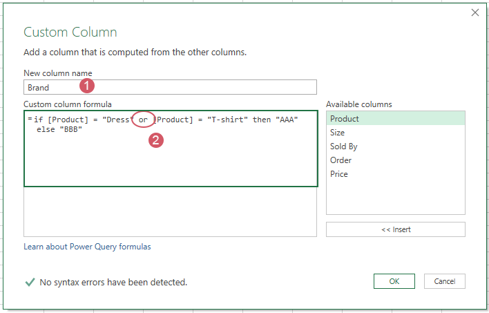
Предположим, у меня есть приведенная ниже таблица, теперь я хочу, чтобы новый столбец отображался следующим образом: если продукт «Платье» или «Футболка», то бренд — «ААА», бренд других продуктов — «ВВВ».

1. Выберите таблицу данных и нажмите Данные > Из таблицы/диапазона , чтобы перейти к Редактор Power Query окно.

2. В открывшемся окне нажмите Добавить столбец > Пользовательский столбец, в открытом Пользовательский столбец диалоговом окне выполните следующие действия:

• Введите имя нового столбца в Имя нового столбца текстовое окно;
• Затем введите приведенную ниже формулу в поле Формула пользовательского столбца пунктом.
• = если [Продукт] = «Платье» или [Продукт] = «Футболка», то «ААА»
  еще «БББ»

3. А затем нажмите OK кнопку, чтобы вернуться к Редактор Power Query окно, и вы получите новый столбец с нужными вам данными, см. скриншот:

4, Наконец, нажмите Главная > Закрыть и загрузить > Закрыть и загрузить чтобы загрузить эти данные на новый лист.

Оператор if с логикой AND

Логика И выполняет несколько логических тестов внутри одного оператора if. Все тесты должны быть истинными, чтобы возвращался истинный результат. Если какой-либо из тестов является ложным, возвращается ложный результат. Синтаксис:

= если логическая_проверка1 и логическая_проверка2 и …, то значение_если_истина иначе значение_если_ложь

Возьмите приведенные выше данные, например, я хочу, чтобы новый столбец отображался как: если продукт «Платье» и заказ больше 300, то дайте скидку 50% от исходной цены; в противном случае сохраните первоначальную цену.

1. Выберите таблицу данных и нажмите Данные > Из таблицы/диапазона , чтобы перейти к Редактор Power Query окно.

2. В открывшемся окне нажмите Добавить столбец > Пользовательский столбец. В открытом Пользовательский столбец диалоговом окне выполните следующие действия:

• Введите имя нового столбца в Имя нового столбца текстовое окно;
• Затем введите приведенную ниже формулу в поле Формула пользовательского столбца пунктом.
• = если [Продукт] = «Платье» и [Заказ] > 300, то [Цена] * 0.5
  еще [Цена]

3, Затем нажмите OK кнопку, чтобы вернуться к Редактор Power Query окно, и вы получите новый столбец с нужными вам данными, см. скриншот:

4. Наконец, вы должны загрузить эти данные в новый рабочий лист, щелкнув Главная > Закрыть и загрузить > Закрыть и загрузить.

Если оператор с логиками ИЛИ и И

Хорошо, предыдущие примеры нам легко понять. Теперь давайте усложним. Вы можете комбинировать И и ИЛИ, чтобы сформировать любое условие, которое вы можете себе представить. В этом типе вы можете использовать скобки в формуле для определения сложных правил.

Возьмите приведенные выше данные в качестве примера. Предположим, я хочу, чтобы новый столбец отображался следующим образом: если продукт «Платье» и его заказ больше 300, или продукт «Брюки» и его заказ больше 300, то показать «A+», иначе отобразите «Другое».

1. Выберите таблицу данных и нажмите Данные > Из таблицы/диапазона , чтобы перейти к Редактор Power Query окно.

2. В открывшемся окне нажмите Добавить столбец > Пользовательский столбец. В открытом Пользовательский столбец диалоговом окне выполните следующие действия:

• Введите имя нового столбца в Имя нового столбца текстовое окно;
• Затем введите приведенную ниже формулу в поле Формула пользовательского столбца пунктом.
• =if ([Продукт] = «Платье» и [Заказ] > 300) или
  ([Товар] = «Брюки» и [Заказ] > 300 )
  потом «А+»
  еще «Другое»

3, Затем нажмите OK кнопку, чтобы вернуться к Редактор Power Query окно, и вы получите новый столбец с нужными вам данными, см. скриншот:

4. Наконец, вы должны загрузить эти данные в новый рабочий лист, щелкнув Главная > Закрыть и загрузить > Закрыть и загрузить.

Аналог функции Excel ИЛИ() в Power Query – List.AnyTrue()

=if <logical test> then <result> else <alternate result>

К сожалению, в Power Query нет функции ИЛИ(). Напомню, чтобы обратиться к списку функций, кликните на ссылку Сведения о формулах Power Query в нижней части диалогового окна Настраиваемый столбец. Вы окажитесь на странице сайта Microsoft с обзором всех функций Power Query. В категории List functions можно найти функцию List.AnyTrue, которая возвращает ИСТИНА, если хоть одно выражение списка истинно. В документации по функции приведено два примера:

Определяет, является ли хотя бы одно из выражений в списке {true, false, 2 > 0} истинным…

List.AnyTrue({true, false, 2>0})

… и возвращает true.

Определяет, является ли хотя бы одно из выражений в списке {2 = 0, false, 2 < 0} истинным…

List.AnyTrue({2 = 0, false, 2 < 0})

… и возвращает false.

Попробуем использовать эту функцию в качестве теста в пользовательском столбце:

    if List.AnyTrue(

      {

        [Column1] = «TRUE»,

        [Sold By] = «FALSE»

      }

    )

    then

      «TRUE»

    else

      «FALSE»

Не забудьте разделить критерии запятыми, а список критериев окружить фигурными скобками, потому что функция List.AnyTrue() в качестве параметра требует список.

Репликация функции Excel И()

Для этих целей в Power Query есть функция List.AllTrue(). Эта функция возвращает истинное значение только в том случае, если каждый логический тест возвращает истинное значение. В Excel щелкните правой кнопкой мыши запрос pqOR –> Дублировать. Переименуйте запрос – pqAND. Если вы удалили столбец Match, удалите этот шаг, чтобы вернуть столбец Match в запрос. Щелкните значок шестеренки рядом с шагом Добавлен пользовательский столбец (для редактирования формулы). Заменить List.AnyTrue на List.AllTrue. Выберите шаг Строки с примененным фильтром.

Хотя в этих примерах мы явно отфильтровали данные на основе столбца Match, самое замечательное в функциях List.AnyTrue и List.AllTrue заключается в том, что вы можете помечать записи без фильтрации. Это добавит вам гибкости при построении более сложной логики, с возможностью сохранения всех исходных данных (чего нельзя получить просто фильтруя столбцы).

Репликация функции SWITCH() Power Pivot

Power Pivot имеет функцию SWITCH(), которая позволяет выполнять логику с несколькими условиями. Функция ищет указанное значение индекса и возвращает соответствующий результат. Эта функция проще, чем несколько уровней вложенных операторов ЕСЛИ(), поэтому полезно реплицировать функцию SWITCH() в Power Query.

Синтаксис этой функции в PowerPivot выглядит следующим образом:

=SWITCH(expression,value_1,result_1,[value_2,result_2],…,[Else])

Допустим, вы выставляете счета клиентам на основе кодированного шаблона, где каждый символ что-то значит. Например, в счете MP010450SP девятый символ может принимать следующие значения:

E = Employee, S = Yacht Club, N = Non-Taxable, R = Restricted, I = Inactive, L = Social, M = Medical, U = Regular

В Excel вы можете построить формулу с многократными вложениями оператора ЕСЛИ или использовать ВПР(). В Power Pivot, это намного проще с функцией SWITCH():

=SWITCH(

[Column],

«E», «Employee»,

«S», «Yacht Club»,

«N», «Non-Taxable»,

«R», «Restricted»,

«I», «Inactive»,

«L», «Social»,

«M», «Medical»,

«U», «Regular»,

«Undefined»

)

Построение функции Power Query SWITCH()

Откройте файл Emulating SWITCH.xIsx. Данные –> Получить данные –> Из других источников –> Пустой запрос. Назовите запрос – fnSWITCH. Главная –> Расширенный редактор. Введите код:

Ключевые части этого кода:

• result_1 – это первая из возможностей, которую вы можете передать в функцию
• return_value_1 – это значение, которое вернет функция, если первое значение = result_1
• Если вам нужно больше значений, вы добавляете запятую после строки {result_1, return_value_1} и вставляете строки {result_2, return_value_2}, {result_3, return_value_3} и т.д.
• Вы можете добавить столько значений, сколько вам нужно
• Если в предоставленном списке нет переданного значения функция вернет текст Undefined (это часть Else конструкции SWITCH).

Используя эту структуру, вы можете изменить функцию fnSWITCH для нашего сценария:

=fnSWITCH(Text.Range([Column1],8,1))

//Помните, что вам нужно начать извлечение текста с символа 8, чтобы получить девятый символ, потому что Power Query начинает отсчет с нуля

//fnSWITCH

Вы не ограничены поиском отдельных символов. Вы можете также искать значения (числа) или более длинные текстовые строки. Просто убедитесь, что ваши параметры всегда вводятся парами между фигурными скобками и имеют запятую в конце строки.

Когда вы закончите вносить изменения в Расширенном редакторе, нажмите кнопку Готово. Главная –> Закрыть и загрузить. Теперь вы можете использовать функцию fnSWITCH для извлечения типа выставленного счета из каждой записи.

Репликация функции Excel ВПР()

Репликация зависит от того, какая версия ВПР/VLOOKUP вам нужна. При поиске точного совпадения репликация может быть получена простым объединением двух таблиц (см. главу 9). Репликация приблизительного соответствия ВПР() требует довольно сложной логики (подробнее о функции ВПР в Excel см. Билл Джелен. Всё о ВПР: от первого применения до экспертного уровня). В примере вы не будете создавать сценарий Power Query с нуля но увидите как он работает. Откройте файл Emulating VLOOKUP.xlsx. В нем есть две таблицы:

Столбцы B:D таблицы данных содержат функции VLOOKUP() соответствующие заголовкам столбцов. Каждый столбец ищет значение, из столбца A для этой строки в таблице подстановки. Столбцы B и D возвращают значение из столбца 2 (G) таблицы подстановки, а столбец C – из столбца 3 (Н). Также обратите внимание, что столбцы B и C возвращают приблизительные совпадения, поскольку четвертый параметр функции VLOOKUP = True или опущен. Столбец D запрашивает точное совпадение (четвертый параметр = False), в результате чего все записи возвращают #N/A, за исключением последней строки.

Давайте поместим сценарий Power Query в файл, а затем посмотрим, как он реплицирует функцию VLOOKUP() Excel. В проводнике Windows кликните на файл pqVLOOKUP.txt Он откроется в Блокноте. Выделите и скопируйте в буфер все содержимое файла. Вернитесь в Excel. Данные –> Получить данные –> Из других источников –> Пустой запрос –> Расширенный редактор. Выделите всю заготовку кода в окне. Ctrl+V (вставив из буфера ранее скопированный код). Нажмите кнопку Готово. Переименуйте функцию pqVLOOKUP. Главная –> Закрыть и загрузить (функции сохраняются только в режиме подключения).

При работе с функцией вам понадобится указатель на таблицу подстановки BandingLevels. Выберите любую ячейку в ней –> Данные –> Из таблицы/диапазона. Главная –> Закрыть и загрузить… –> Только создать подключение.

Теперь всё готово, чтобы посмотреть, как это работает. Удалите из таблицы данных (DataTable) все формулы Excel (ячейки В3:D10). Выберите любую ячейку в таблице DataTable –> Данные –> Из таблицы/диапазона. Щелкните правой кнопкой мыши столбец Values –> Удалить другие столбцы:

Рис. 22.8. Запрос готов к использованию функции pqVLOOKUP

Чтобы проверить, работает ли функция PQ VLOOKUP для вас, вы можете попробовать повторить следующую формулу: =VLOOKUP ([Values], BandingLevels, 2, true)

Для этого можно выполнить следующие действия:

Добавление столбца –> Настраиваемый столбец. Назовите столбец 2,True. Используйте формулу:

=pqVLOOKUP([Values],BandingLevels,2,true)

Рис. 22.9. Репликация VLOOKUP() с четвертым параметром равным true

Снова перейдите на вкладку Добавление столбца –> Настраиваемый столбец. Назовите столбец 3,default. Используйте формулу:

=pqVLOOKUP([Values],BandingLevels,3)

Рис. 22.10. Репликация VLOOKUP() с опущенным четвертым параметром (по умолчанию = true, приблизительное совпадение)

Теперь определите точное совпадение со вторым столбцом таблицы подстановки. Добавление столбца –> Настраиваемый столбец. Назовите его 2,false. Используйте формулу:

=pqVLOOKUP([Values],BandingLevels,2,false)

Рис. 22.11 Репликация VLOOKUP() с точным совпадением

Несмотря на то, что вы можете использовать эту функцию для эмуляции точного соответствия VLOOKUP(), лучше этого не делать, а воспользоваться объединением таблиц. Завершите запрос. Главная –> Закрыть и загрузить.

Вы должны знать об одном незначительном отличии между функцией VLOOKUP() Excel и pqVLOOKUP Power Query: значение #N/A, возвращаемое pqVLOOKUP, на самом деле является текстом, а не значением ошибки. Поскольку истинную ошибку #N/A в Power Query вернуть нельзя.

Понимание функции pqVLOOKUP

Взгляните на код:

Код довольно длинный и сложный, и он использует множество трюков, но основная методология следующая:

1. Втяните таблицу подстановки в Power Query.
2. Отсортируйте ее по убыванию по первому столбцу.
3. Удалите все записи, превышающие искомое значение.
4. Верните значение в запрошенном столбце таблицы данных для первой оставшейся записи, если не указано точное соответствие.
5. Если было указано точное соответствие, проверьте, соответствует ли возврат. Если это так, верните значение. Если это не так, верните #N/A.

Для каждого параметра функции в первой строке кода объявлен тип данных. Это делается для предотвращения проблем, если случайно в таблице подстановки заголовки будут числами.

Переменная approximate_match определена как необязательная (optional); пользователь может игнорировать ее.

Переменная matchtype проверяет, был ли указан тип соответствия. Если он был указан, именно он присваивается переменной matchtype, если не был указан (approximate_match равен null), то присваивается значение true.

Имя возвращаемого столбца извлекается путем просмотра заголовков столбцов таблицы, разбиения их на список записей и извлечения записи, индекс которой соответствует запрошенному столбцу (на 1 меньше, так как отсчет начинается с 0).

Данные сортируются в порядке убывания, в зависимости от столбца для поиска. Все записи, превышающие запрошенное значение, удаляются (путем выбора всех строк, где значение меньше или равно искомому значению).

Если строк не осталось, возвращается #N/А, если есть хотя бы одна строка, возвращается первая запись в столбце поиска. Этот результат может быть позже проверен, чтобы увидеть, соответствует ли он искомой записи (что важно для точного соответствия).

Затем вычисляется приблизительное значение соответствия, даже если было запрошено точное соответствие. Если в наборе данных нет строк, сохраняется результат #N/A; в противном случае из возвращаемого столбца извлекается ближайшее значение.

Последний тест проверяет тип запрошенного соответствия. Если это приблизительное совпадение, то возвращается самое близкое совпадение (которое может быть #N/A). Если тип соответствия был точным, код вернет #N/A вместо ближайшего соответствия, если значение столбца подстановки не соответствует точно искомому значению.

Power BI offers top-of-the-line features for both beginners and power users. With a relatively low learning curve and its strong integration capabilities with Microsoft Apps, Power BI is a fantastic data visualization tool to explore your data and create engaging reports. Within Power BI is a lightweight tool called Power Query to transform and shape data tables. 

One such data shaping tool in Power BI is Power Query IF Statement, which makes data transformation easy and allows you to compare values. Using Power Query IF statements, Power BI users can slice data fields, retain relevant information, derive and create new parameters, and sort data for more detailed analysis. 

This guide introduces you to Power Query, a self-service data preparation tool for the Power BI family, Power Query IF statements with conditional and custom columns, and finally common operators that you can use to create conditional Power Query IF statements. 

Table of Contents

• What is Power BI?
• Business Benefits of Using Power BI
• What is a Power Query?
• What is a Power Query IF Statement?
• How to Use Power Query IF Statements?
• Types of Power Query IF Statements
• Common Operators in Power Query IF Statements
• Conclusion

What is Power BI?

The Gartner Magic Quadrant Report has rewarded Microsoft Power BI as the leader in the Business Intelligence industry for 14 consecutive years. Clearly, that explains a lot about Power BI.

Power BI is a Microsoft Business Intelligence suite to analyze data and share insights. It features capabilities such as:

• Dataset filtration,  
• Visual-based data discovery, 
• Interactive dashboards, 
• Augmented analytics,
• Natural Language Q & A Question Box,
• Office 365 App Launcher, and many more.

Microsoft Power BI runs on desktop and mobile, on the cloud, which means your teams can collate, manage, and analyze data from anywhere. Power BI allows you to upload data from multiple sources like Excel, CSV, SQL Server, MySQL database, PDF, Access, XML, JSON, and a plethora more. 

Microsoft Power BI collects, analyzes, and transforms your data into actionable insights. These insights are frequently provided using aesthetically appealing and simple-to-understand charts and graphs, which enables faster decision-making in your organization. When combined with Azure Cloud, Power BI can accelerate big data preparation and analysis and reduce your time to decision planning tremendously.

For more information on Power BI, do check out Understanding Microsoft Power BI: A Comprehensive Guide. If your organization uses Microsoft Azure cloud to store, manage and access information, you can combine your Azure cloud with Power BI using this guide – Connect Azure to Power BI: A Comprehensive Guide.

Business Benefits of Using Power BI

• Interactive & Easy-to-Use Interface: Nothing can be more beneficial than a simple-to-use interface with a drag and drop functionality that lets you create data visualizations using a few clicks. Microsoft Power BI enables everyone at every level of your organization to make confident decisions using up-to-the-minute analytics.
• Multiple Dataset Sources: Using Power BI, you can import data from a plethora of data sources, with support for both structured and unstructured data.
• Industry-leading AI: Microsoft’s strong base in artificial intelligence enables Power BI users to prepare data, build machine learning models, and find insights quickly from both structured and unstructured data.
• Exceptional Excel Integration: With Power BI, your users can easily collect, analyze, publish, and share Excel business data. Excel queries, data models, and reports can be readily connected to Power BI Dashboards by anybody who is acquainted with Office 365.
• Real-time Stream Analytics: Power BI fetches real-time data insights into your data visualizations to keep your teams up-to-date and ready to make the right decisions. 
• Turn Insights to Action: Using Microsoft Power Platform, your teams can deliver actions quickly by combining Power BI with Power Apps and Power Automate. Using Microsoft’s strong integration, your users can easily build business applications and automate workflows.

What is a Power Query?

Power Query is an intelligent data transformation and data preparation tool offered as part of Microsoft Excel and Microsoft Power BI. Power Query simplifies the process of importing data from multiple file formats like Excel tables, CSV files, database tables, webpages, etc. and allows you to transform your data into the right shape and condition for better analysis. 

Once you have set up your Power Query operations, you don’t have to perform the same set of processes again on your new data. Using Power Query, you can easily set up and automate the same data transformation processes and yield the same data outputs as done previously.

Power Query functionality in Microsoft Power BI allows you to perform extensive data transformations such as:

• Deleting unnecessary columns, rows, or blanks.
• Data type conversions – text, numbers, dates.
• Splitting or merging columns.
• Using Power Query IF statements to sort & filter columns.
• Adding new calculated columns.
• Aggregating or summarizing data, and many more.

What is a Power Query IF Statement?

Power Query IF statement is one of the many ways to transform your data. Similar to the IF statement in Microsoft Excel, the IF statement Power Query function checks a condition and returns a value depending on whether the result is “true” or “false”.

In Power BI, IF statements can be used as both DAX functions and Power Query conditional columns. In this guide, we’ll be confining ourselves to the IF statement in Power Query. For the DAX version of the Power BI IF Statement, we have a separate detailed guide that you can check out here – How to Use Power BI IF Statement: 3 Comprehensive Aspects. You can avail more information on DAX functions in Power BI here- Understanding DAX Power BI: A Comprehensive Guide.

How to Use Power Query IF Statements?

Power Query offers you two options to write Power Query IF statements:

• Using Conditional Column For Basic Power Query IF Statement Logic.
• Using Custom Column For More Advanced IF Statement Power Query Logic.

Power Query IF Statement: Syntax

If you would like to write the IF statement Power Query Command in your formula editor (using a custom column), you can refer to the following syntax for defining your conditional expressions.

if “if-condition” then “true-expression” else “false-expression”

Please note that Power Query IF statements are case-sensitive and the words if…then…else are written in lowercase. 

Let’s look at how to use Power Query IF statements with the Conditional Column Feature.

Using Conditional Column For Basic Power Query IF Statement Logic

With the conditional column feature, Power Query IF statements like—Power Query IF THEN, Power Query IF OR, Power Query IF AND, and Power Query IF NULL becomes much easier to define. Even more so than the Excel equivalents. 

To use the conditional column, you can visit Add Column > Conditional Column in your Power Query pane. This approach of Power Query IF statements allows you to define basic-if statements. 

Consider this sales data example to help understand the conditional column feature for basic Power Query IF Statement logic. 

The sample file used for this example can be found here – Power Query IF Statement-Example File. You can import this file to your Power Query editor by selecting any cell in this table and clicking Data -> From Table/Range to load the data into Power Query.

In this example, we are required to add a new column called Incentive based on the following conditions:

• If the Sales Value is > $6500, the incentive given will be $300.
• If the Sales Value is < $6500, the incentive given will be $200.

To use the Power Query editor window, we first need to enable editing for your sales data table. For that, visit Home > Edit Queries.

Now, visit the tab Add Column > Conditional Column to define your Power Query IF statement and insert the new column “incentive”. A new window will appear as shown below.

The next set of tasks is fairly simple. All you have to do is define your Power Query IF statement, using the drop-down options in the window.

Type in your new column name under the heading New column name. Since we are offering an incentive of $300 for sales value > $65000, we’ll establish our IF statement Power Query conditional as:

If Sales Value is greater than 6500 then Output is 300 Else 200. 

Which translates to:

Reasonably straightforward right. You can use this menu to define and use basic IF statement logic. The available options and their input fields are as follows:

• New Column Name: Defines the column name for your new column.
• Column Name: The column name which is evaluated against your Power Query IF statement.
• Operator: Mathematical operation which compares text, numbers, or date data type present in your column name using less than, greater than, equal to operations, etc.
• Value: Parameter or value against which the comparison is made.
• Output: Value or parameter returned when a condition is met.
• Else: Value or parameter returned when a condition is not met (when previous conditions get false).

Click OK to apply changes and add a new column, “incentive” to your sales table. Your first conditional column feature for basic Power Query IF statement logic is now complete. Your new column will be visible as soon as you leave your conditional column window.

Please note that the conditional column feature supports basic Power Query IF statement logic; the ones which can be “fairly” expressed as a single sentence in English. For more granular and complex conditional statements, we recommend you take advantage of the custom column feature or formula editor, as described in the next section.

Using Custom Column For More Advanced IF Statement Power Query Logic

Your usual day data table transformations won’t be as easy as previously described. Even simple Power Query IF statement conditions like dividing A by B when the result is less than C would require you to write an IF statement in the Power Query editor. 

Custom column option can be accessed in your Power Query under the tab Add Column > Custom Column. When you click on the Custom Column option, a new window will open with space to define and write your new IF conditional expressions.

Since our daily conditional expressions are more complex, let’s revamp our original problem to reflect a pragmatic setting. 

Let’s say you own a business, and you want to incentivize your sales representatives based on their locations. You decided to reward your sales representatives residing in the South region who’ve produced more than $6500 sales value with a $400 dollar prize. For the rest, the conditions remain the same.

Our Power Query IF statement for a new condition, if stated in plain English, would look like:

If Sales Value is greater than 6500 and Region is South, then Output is 400

Else Sales Value is greater than 6500, then Output is 300. 

Else 200.

Putting this into our Power Query editor, with if..then..else in lowercase, we get:

To distinguish the difference between new incentive plans and old incentive plans, we have named this new custom column as Incentive 2, as opposed to the original Incentive 1.

Here’s how both new columns will stack up. You can see the change in rewards, for sales representatives like Roshan, who was getting $300 with the original scheme and $400 with the new incentive scheme.

Hit Home > Close and Apply to save your changes. You have now successfully used a custom column for more advanced IF statement Power Query logic.

Types of Power Query IF Statements

Power Query IF statements come in different forms:

• Power Query IF OR
• Power Query IF AND
• Power Query IF NULL
• Power Query nested IF

Power Query IF OR Statement

Power Query IF OR specifies two conditions to be evaluated (separately) for stating them as true or yielding the desired output. The others are stated false and returned with a different value or parameter. In other terms,

= if something is true or something else is true then “true” else “false”

Extending on our previous sales data, if you wish to incentivize sales representatives operating in south or central regions with $350, and the rest with $200, you can run a Power Query IF OR query as follows: 

=if [Region] = "South" or [Region] = "Central" then 350 else 200

Power Query IF AND Statement

Power Query IF AND specifies two conditions to be evaluated (simultaneously) for stating them as true or yielding the desired output. The others are stated false and returned with a different value or parameter. In other terms,

= if something is true and something else is true then “true” else “false”

If you wish to incentivize sales representatives operating in south region having sales value of more than $6500 with $450, and the rest with $200, you can run a Power Query IF AND query as follows: 

=if [Region] = "South" and [Sales Value] > 6500 then 450 else 200

Another example can be if you wish to provide a bonus to sales representatives operating in the central region having a sales value of more than $6500 with prize money of 0.5% of sales value, then your IF AND query will look like this:

=if [Region] = "Central" and [Sales Value] > 6500 then [Sales Value] * 0.005 else 0

Power Query IF NOT Statement

Power Query IF NOT checks a condition if it’s true or not. If it’s TRUE, the operator returns FALSE, and if given FALSE, the operator returns TRUE. So, basically, it will always return a reverse logical value.

= if not something is true then “true” else “false”

Let us assume you just want to reverse what you did in your earlier example. You wish to award bonuses to all the other sales representatives who are not residing in the south region having sales value of more than $6500. Using the IF NOT statement, you can run a Power Query conditional statement as: 

=if not ([Region] = "South" and [Sales Value] > 6500) then 450 else 200

Power Query Nested IF Statement

Analogous to Microsoft Excel, nested IF statements are IF statements contained within other IF statements. These nested IF statements can be used to return a TRUE or FALSE, which can be further used as inputs to other IF statements. 

Here’s an example to clarify nested IF statements in Power Query. 

Suppose you wish to boost sales efforts in the central region by rewarding a bonus of 0.5%, in the west region by rewarding a bonus of 0.3%, and in the south region by rewarding a bonus of 0.2% of sales value. For such a case, your nested IF statement would look like this:

= if [Region] = “Central” then [Sales Value] * 0.05
  if [Region] = “West” then [Sales Value] * 0.03
  if [Region] = “South” then [Sales Value] * 0.02

To make nested Power Query IF statements work, place the second if statement after the first otherwise clause. The formula in this example is created with space and line breaks. This increases readability while still performing appropriately.

Common Operators in Power Query IF Statements

Till this point, we’ve discussed basic logic IF statements to simply compare two quantities. Power Query IF statements offer a plethora of mathematical operators to help tailor-craft your conditional statements as per your needs. These include:

• “=” is equal to
• “<>” is not equal to
• “>=” is greater than or equal to
• “<=” is less than or equal to
• “>” is greater than
• “<” is less than
• “+” for sum
• “-” for difference
• “*” for product
• “/” for quotient
• “+x” for unary plus
• “-x” for negation

These mathematical operators can be used while writing your IF conditional statements in Power Query editor (custom column method).

Recommended Blogs

• List of DAX Functions for Power BI: 8 Popular Function Types
• Ultimate Guide on Power BI Visuals: 20+ Types to Use in 2022
• Setting Up A Power BI Data Gateway: 3 Easy Steps
• A Complete List Of Power BI Data Sources Simplified 101

Conclusion

We hope this comprehensive piece provided a lucid explanation around Power Query IF statements, and that you are now ready to write and use your own customized IF conditional statements. We showed you two ways to use Power Query IF statements—one using conditional column which is useful for basic IF statement logic and, the other using custom column which is valuable when using advanced IF statement logic.

Power Query in Power BI constructive tool for importing data from a variety of sources. While Power Query is just limited to Excel sheets and CSV file formats, why not import data from Databases like MySQL and PostgreSQL, SaaS applications like Mailchimp, Zendesk, and CRMs like Salesforce, and HubSpot to Power BI? Wondering how this is possible?

Hevo Data is a No-Code and Zero Data Loss Solution that supports data ingestion from multiple sources be it your frequently used databases and SaaS applications like MySQL, PostgreSQL, Salesforce, Mailchimp, Asana, Trello, Zendesk, and other 100+ data sources. Hevo migrates your data to a secure central repository like a Data Warehouse in minutes with just a few simple clicks.

Using Hevo is simple, and you can set up a Data Pipeline in minutes without worrying about any errors or maintenance aspects. Hevo also supports advanced data transformation and workflow features to mold your data into any form before loading it to the target database.

Visit our Website to Explore Hevo

Hevo lets you migrate your data from your favorite applications to any Data Warehouse of your choice like Amazon Redshift, Snowflake, Google BigQuery, or Firebolt, within minutes to be analyzed in Power BI.

Why not try Hevo and the action for yourself? Sign Up here for a 14-day free trial and experience the feature-rich Hevo suite first hand. You can also check out our pricing plans to choose the best-matched plan for your business needs. 

Have more ideas or Power BI features you would like us to cover? Drop a comment below to let us know.