Код
Хэмминга относится к классу линейных
кодов и представляет собой систематический
код – код, в котором информационные и
контрольные биты расположены на строго
определенных местах в кодовой комбинации.
Код
Хэмминга, как и любой (n,
k)-
код, содержит к
информационных и m
= n-k
избыточных (проверочных) бит.
Избыточная
часть кода строится т. о. чтобы можно
было при декодировании не только
установить наличие ошибки но, и указать
номер позиции в которой произошла ошибка
, а значит и исправить ее, инвертировав
значение соответствующего бита.
Существуют
различные методы реализации кода
Хэмминга и кодов которые являются
модификацией кода Хэмминга. Рассмотрим
алгоритм построения кода для исправления
одиночной ошибки.
1.
По заданному количеству информационных
символов — k,
либо информационных комбинаций N
= 2k
, используя соотношения:
n
= k+m, 2n
(n+1)2k
и
2m
n+1 (14)
m
= [log2
{(k+1)+
[log2(k+1)]}]
вычисляют
основные параметры кода n
и m.
2.
Определяем рабочие и контрольные позиции
кодовой комбинации. Номера контрольных
позиций определяются по закону 2i,
где
i=1,
2, 3,… т.е. они равны 1, 2, 4, 8, 16,… а остальные
позиции являются рабочими.
3.
Определяем значения контрольных разрядов
(0 или 1 ) при помощи многократных проверок
кодовой комбинации на четность. Количество
проверок равно m
= n-k.
В каждую проверку включается один
контро-льный и определенные проверочные
биты. Если результат проверки дает
четное число, то контрольному биту
присваивается значение -0, в противном
случае — 1. Номера информационных бит,
включаемых в каждую проверку, определяются
по двоичному коду натуральных n
–чисел
разрядностью – m
(табл.
1, для m
= 4)
или при помощи проверочной матрицы
H(mn),
столбцы которой представляют запись в
двоичной системе всех целых чисел от 1
до 2k
–1
перечисленных в возрастающем порядке.
Для
m = 3
проверочная матрица имеет вид
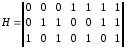 .
.
(15 )
Количество
разрядов m
— определяет количество проверок.
В
первую проверку включают коэффициенты,
содержащие 1 в младшем (первом) разряде,
т. е. b1,
b3,
b5
и т. д.
Во
вторую проверку включают коэффициенты,
содержащие 1 во втором разряде, т. е. b2,
b3,
b6
и т. д.
В
третью проверку — коэффициенты которые
содержат 1 в третьем разряде и т. д.
Таблица
1
|
Десятичные
(номера
кодовой |
Двоичные |
||
|
3 |
2 |
1 |
|
|
1 2 3 4 5 6 7 |
0 0 0 1 1 1 1 |
0 1 1 0 0 1 1 |
1 0 1 0 1 0 1 |
Для
обнаружения и исправления ошибки
составляются аналогичные проверки на
четность контрольных сумм, результатом
которых является двоичное (n-k)
-разрядное число, называемое синдромом
и указывающим на положение ошибки, т.
е. номер ошибочной позиции, который
определяется по двоичной записи числа,
либо по проверочной матрице.
Для
исправления ошибки необходимо
проинвертировать бит в ошибочной
позиции. Для исправления одиночной
ошибки и обнаружения двойной используют
дополнительную проверку на четность.
Если при исправлении ошибки контроль
на четность фиксирует ошибку, то значит
в кодовой комбинации две ошибки.
Схема
кодера и декодера для кода Хэмминга
приведена на рис. 1.
Пример
1.
Построить код Хемминга для передачи
сообщений в виде последовательности
десятичных цифр, представленных в виде
4 –х разрярных двоичных слов. Показать
процесс кодирования, декодирования и
исправления одиночной ошибки на примере
информационного слова 0101.
Решение:
1.
По заданной длине информационного слова
(k
= 4),
определим количество контрольных
разрядов m,
используя соотношение:
m
= [log2
{(k+1)+
[log2(k+1)]}]=[log2
{(4+1)+
[log2(4+1)]}]=3,
при
этом n
= k+m = 7,
т. е. получили (7, 4) -код.
2.
Определяем номера рабочих и контрольных
позиции кодовой комбинации. Номера
контрольных позиций выбираем по закону
2i
.
Для
рассматриваемой задачи (при n
= 7)
номера контрольных позиций равны 1, 2,
4. При этом кодовая комбинация имеет
вид:
b1
b2
b3
b4
b5
b6
b7
к1
к2
0
к3
1
0 1
3.
Определяем значения контрольных разрядов
(0 или 1), используя проверочную матрицу
(5).
Первая
проверка:
k1
b3
b5
b7
= k1011
будет четной при k1
=
0.
Вторая
проверка:
k2
b3
b6
b7
= k2001
будет четной при k2
=
1.
Третья
проверка:
k3
b5
b6
b7
= k3101
будет четной при k3
=
0.
1
2 3 4 5 6 7
Передаваемая
кодовая комбинация: 0 1 0 0 1 0 1
Допустим
принято: 0 1 1 0 1 0 1
Для
обнаружения и исправления ошибки
составим аналогичные про-верки на
четность контрольных сумм, в соответствии
с проверочной матрицей результатом
которых является двоичное (n-k)
-разрядное число, называемое синдромом
и указывающим на положение ошибки, т.
е, номер ошибочной позиции.
1)
k1
b3
b5
b7
= 0111 = 1.
2)
k2
b3
b6
b7
= 1101 = 1.
-
k3
b5
b6
b7
= 0101 = 0.
Сравнивая
синдром ошибки со столбцами проверочной
матрицы, определяем номер ошибочного
бита. Синдрому 011 соответствует третий
столбец, т. е. ошибка в третьем разряде
кодовой комбинации. Символ в 3 -й позиции
необходимо изменить на обратный.
Пример
2.
Построить код Хэмминга для передачи
кодовой комбинации 1 1 0 1 1 0 1 1. Показать
процесс обнаружения и исправления
ошибки в соответствующем разряде кодовой
комбинации.
Решение:
Рассмотрим
алгоритм построения кода для исправления
одиночной ошибки.
1.
По заданной длине информационного слова
(k
= 8)
, используя соотношения вычислим основные
параметры кода n
и m.
m
= [log2
{(k+1)+
[log2(k+1)]}]=[log2
{(9+1)+
[log2(9+1)]}]=4,
при
этом n
= k+m = 12,
т. е. получили (12, 8)-код.
2.
Определяем номера рабочих и контрольных
позиции кодовой комбинации. Номера
контрольных позиций выбираем по закону
2i
.
Для
рассматриваемой задачи (при n
= 12)
номера контрольных позиций равны 1, 4,
8.
При
этом кодовая комбинация имеет вид:
b1
b2
b3
b4
b5
b6
b7
b8
b9
b10
b11
b12
к1
к2
1
к3
1
0 1 к4
1
0 1 1
3.
Определяем значения контрольных разрядов
(0 или 1) путем много-кратных проверок
кодовой комбинации на четность. Количество
проверок равно m
= n-k.
В каждую проверку включается один
контрольный и определенные проверочные
биты.
Номера
информационных бит, включаемых в каждую
проверку определяется по двоичному
коду натуральных n-чисел
разрядностью — m.
0001
b1
Количество разрядов m — определяет
количество прове-
0010
b2
верок.
0011
b3
1) к1
b3
b5
b7
b9
а11
=
к111111
=>
0100
b4
четная
при к1=1
0101
b5
2)
к2
b3
b6
b7
b10
b11=
к210101
=>
0110
b6
четная при к2=1
0111
b7
3)
к3
b5
b6
b7
b12
=
к31011=>
1000
b8
четная
при к3=1
1001
b9
4) к4
b9
b10
b11
b12
=
к11011
=>
1010
b10
четная
при к4=1
1011
b11
1100
b12
Передаваемая
кодовая комбинация: 1 2 3 4 5 6 7 8 9 10 11 12
1
1 1 1 1 0 1 1 1 0 1 1
Допустим,
принято: 1 1 1 1 0 0 1 1 1 0 1 1
Для
обнаружения и исправления ошибки
составим аналогичные про-верки на
четность контрольных сумм, результатом
которых является двоичное (n-k)
-разрядное число, называемое синдромом
и указывающим на положение ошибки, т.
е. номер ошибочной позиции.
1)
к1
b3
b5
b7
b9
b11
=
110111 =1
2)
к2
b3
b6
b7
b10
b11
=
110101 =0
3)
к3
b5
b6
b7
b12
=
10011 =1
4)
к4
b9
b10
b11
b12
=
11011 =0
Обнаружена
ошибка в разряде кодовой комбинации с
номером 0101, т. е. в 5 -м разряде. Для
исправления ошибки необходимо
проинвертировать 5 -й разряд в кодовой
комбинации.
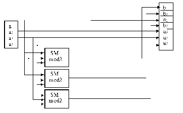
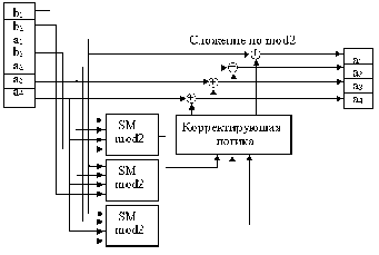
Рис.
1. Схема кодера —а
и декодера –б
для простого (7, 4) кода Хэмминга
Рассмотрим
применение кода Хэмминга. В ЭВМ код
Хэмминга чаще всего используется для
обнаружения и исправления ошибок в ОП,
памяти с обнаружением и исправлением
ошибок ECC Memory (Error Checking and Correcting). Код
Хэмминга используется как при параллельной,
так и при последовательной записи. В
ЭВМ значительная часть интенсивности
потока ошибок приходится на ОП. Причинами
постоянных неисправностей являются
отказы ИС, а случайных изменение
содержимого ОП за счет флуктуации
питающего напряжения, кратковременных
помех и излучений. Неисправность может
быть в одном бите, линии выборки разряда,
слова либо всей ИС. Сбой может возникнуть
при формировании кода (параллельного),
адреса или данных, поэтому защищать
необходимо и то и др. Обычно дешифратор
адреса встроен в м/схему и недоступен
для потребителя. Наиболее часто ошибки
дают ячейки памяти ЗУ, поэтому главным
образом защищают записываемые и
считываемые данные.
Наибольшее
применение в ЗУ нашли коды Хэмминга с
dmin=4,
исправляющие одиночные ошибки и
обнаруживающие двойные.
Проверочные
символы записываются либо в основное,
либо специальное ЗУ. Для каждого
записываемого информационного слова
(а не байта, как при контроле по паритету)
по определенным правилам вычисляется
функция свертки, результат которой
разрядностью в несколько бит также
записывается в память. Для 16 -ти разрядного
информационного слова используется 6
дополнительных бит (32- 7 бит, 64 –8 бит).
При считывании информации схема контроля,
используя избыточные биты, позволяет
обнаружить ошибки различной кратности
или исправить одиночную ошибку. Возможны
различные варианты поведения системы:
-
автоматическое
исправление ошибки без уведомления
системы;
—
исправление однократной ошибки и
уведомление системы только о многократных
ошибках;
—
не исправление ошибки, а только уведомление
системы об ошибках;
Модуль
памяти со встроенной схемой исправления
ошибок –EOS 72/64 (ECC on Simm). Аналог микросхема
к 555 вж 1
-это 16 разрядная схема с обнаружением
и исправлением ошибок (ОИО) по коду
Хэмминга (22, 16), использование которой
позволяет исправить однократные ошибки
и обнаружить все двух кратные ошибки в
ЗУ.
Избыточные
(контрольные) разряды позволяют обнаружить
и исправить ошибки в ЗУ в процессе записи
и хранения информации.
В
составе ВЖ-1 используются 16 информационных
и 6 контрольных разрядов. (DB — информационное
слово, CB — контрольное слово).
При
записи осуществляется формирование
кода, состоящего из 16 информационных и
6 контрольных разрядов, представляющих
результат суммирование по модулю 2
восьми информационных разрядов в
соответствии с кодом Хэмминга.
Сформированные контрольные разряды
вместе с информационными поступают на
схему и записываются в ЗУ.
(22,16)
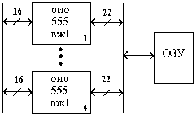
4
схе(72,64)
Рис.2.
Схема контроля
При
считывании шестнадцатиразрядное слово
декодируется, восстанавливаясь вместе
с 6 разрядным словом контрольным,
поступают на схему сравнения и контроля.
Если достигнуто равенство всех контрольных
разрядов и двоичных слов, то ошибки нет.
Любая
однократная ошибка в 16 разрядном слове
данных изменяет 3 байта в 6 разрядном
контрольном слове. Обнаруженный ошибочный
бит инвертируется.
Соседние файлы в предмете [НЕСОРТИРОВАННОЕ]
- #
- #
- #
- #
- #
- #
- #
- #
- #
- #
- #
Содержание
Раздел разработан в 2010 г. при поддержке компании RAIDIX
Для понимания материалов настоящего раздела крайне желательно ознакомиться с разделом КОДИРОВАНИЕ
.
Код Хэмминга
Будем рассматривать двоичные коды, т.е. упорядоченные наборы (строки) $ (x_1,dots,x_{n}) $ из $ n_{} $ чисел $ {x_1,dots,x_n}subset {0,1} $. Множество таких наборов, рассматриваемое вместе с операцией умножения на константы $ 0_{} $ или $ 1_{} $ и операцией поразрядного сложения по модулю $ 2_{} $:
$$ (x_1,dots,x_n)oplus (y_1,dots,y_n)=(x_1oplus y_1 ,dots,x_noplus y_n ) =
$$
$$ = (x_1+y_1 pmod{2},dots,x_n+y_n pmod{2}) $$
образует линейное пространство, которое мы будем обозначать $ mathbb V^n $, а собственно составляющие его наборы будем называть векторами; причем, для определенности, именно векторами-строками. Это пространство состоит из конечного числа векторов: $ operatorname{Card} (mathbb V^n)=2^n $.
Расстояние Хэмминга
Расстоянием Хэмминга между двумя векторами $ B=(b_1,dots,b_n) $ и $ C=(c_1,dots,c_n) $ из $ mathbb V^n $ называется число разрядов, в которых эти слова отличаются друг от друга; будем обозначать его $ rho(B,C) $.
?
Доказать, что
$ rho(B,C)= displaystyle sum_{j=1}^n left[ (1-b_j)c_j+ (1-c_j)b_j right] $ .
Весом Хэмминга вектора $ B=(b_1,dots,b_n) $ называется число его отличных от нуля координат, будем обозначать его $ w(B) $. Таким образом1)
$$ w(B)= b_1+dots+b_n, qquad rho(B,C)=|b_1-c_1|+dots+ |b_n-c_n|=w(B-C) . $$
Расстояние Хэмминга является метрикой в пространстве $ mathbb V^n $, т.е. для любых векторов $ {X_1,X_2,X_3} subset mathbb V^n $ выполняются свойства
1.
$ rho(X_1,X_2) ge 0 $, и $ rho(X_1,X_2) = 0 $ тогда и только тогда, когда $ X_1=X_2 $;
2.
$ rho(X_1,X_2) = rho(X_2,X_1) $;
3.
$ rho(X_1,X_3)le rho(X_1,X_2)+ rho(X_2,X_3) $ («неравенство треугольника»).
Пусть теперь во множестве $ mathbb V^n $ выбирается произвольное подмножество $ mathbb U $, содержащее $ s_{} $ векторов: $ mathbb U={ U_1,dots,U_s } $. Будем считать эти векторы кодовыми словами, т.е. на вход канала связи будем подавать исключительно только эти векторы; само множество $ mathbb U $ будем называть кодом. По прохождении канала связи эти векторы могут зашумляться ошибками. Каждый полученный на выходе вектор будем декодировать в ближайшее (в смысле расстояния Хэмминга) кодовое слово множества $ mathbb U $. Таким образом, «хорошим» кодом — в смысле исправления максимального числа ошибок — может считаться код $ mathbb U $, для которого кодовые слова далеко отстоят друг от друга. С другой стороны, количество кодовых слов $ s_{} $ должно быть достаточно велико, чтобы делать использование кода осмысленным; во всяком случае, будем всегда считать $ s>1 $.
Минимальное расстояние между различными кодовыми словами кода $ mathbb U $, т.е.
$$ d=min_{{j,k}subset {1,dots,s } atop jne k} rho (U_j,U_k) $$
называется кодовым расстоянием кода $ mathbb U $; будем иногда также писать $ d(mathbb U) $.
Т
Теорема. Код $ mathbb U $ с кодовым расстоянием $ d_{} $
a) способен обнаружить от $ 1_{} $ до $ d-1 $ (но не более) ошибок;
б) способен исправить от $ 1_{} $ до $ leftlfloor displaystyle frac{d-1}{2} rightrfloor $ (но не более) ошибок. Здесь $ lfloor rfloor $ — целая часть числа.
Доказательство. Если $ U_1 $ — переданное кодовое слово, а $ V_{} $ — полученный на выходе с канала вектор с $ tau_{} $ ошибками, то $ rho(U_1,V)=tau $. Мы не сможем обнаружить ошибку если $ V_{1} $ совпадет с каким-то другим кодовым словом $ U_2 $, т.е. при условии $ rho(U_2,V)=0 $. Оценим
$ rho(U_2,V) $ при условии, что $ tau le d-1 $. По неравенству треугольника
3
получаем
$$ rho(U_2,V) ge rho(U_1,U_2)-rho(U_1,V) ge d-tau ge 1>0 . $$
Для доказательства части б) предположим, что $ 2,tau le d-1 $. Тогда те же рассуждения приведут к заключению
$$ rho(U_2,V) ge d-tau ge (2,tau+1)-t > tau = rho(U_1,V) , $$
т.е. вектор $ V_{} $ ближе к $ U_1 $, чем к любому другому кодовому слову.
♦
П
Пример. Код Адамара строится на основании матрицы Адамара — квадратной матрицы, элементами которой являются только числа $ {+1,-1} $; при этом ее строки (как, впрочем, и столбцы) попарно ортогональны. Так, матрица Адамара порядка $ 8_{} $ —
$$
H=left(
begin{array}{rrrrrrrr}
1 & 1 & 1 & 1 & 1 & 1 & 1 & 1 \
-1 & 1 &-1 & 1 & -1 & 1 &-1 & 1\
1 & 1 & -1 & -1 & 1 & 1 & -1 & -1 \
-1 & 1 & 1 & -1 & -1 & 1 & 1 & -1 \
1 & 1 & 1 & 1 & -1 & -1 & -1 & -1 \
-1 & 1 &-1 & 1 & 1 & -1 &1 & -1\
1 & 1 & -1 & -1 & -1 & -1 & 1 & 1 \
-1 & 1 & 1 & -1 & 1 & -1 & -1 & 1
end{array}
right) .
$$
Код строится следующим образом. Берутся строки матрицы $ H_{} $ и умножаются на $ +1 $ и на $ -1 $; в каждой строке множества
$$ H^{[1]},H^{[2]},dots,H^{[8]},-H^{[1]},-H^{[2]},dots,-H^{[8]} $$
производится замена $ +1 to 0, -1 to 1 $. Получаются $ 16 $ векторов
$$
(00000000), (10101010), (00110011), (10011001), (00001111), (10100101), (00111100),
(10010110),
$$
$$
(11111111), (01010101), (11001100), (01100110), (11110000), (01011010), (11000011),
(01101001),
$$
которые обозначим $ U_1,dots,U_8,U_{-1},dots,U_{-8} $.
Поскольку строки $ pm H^{[j]} $ и $ pm H^{[k]} $ ортогональны при $ jne k_{} $ и состоят только из чисел $ pm 1 $, то ровно в половине своих элементов они должны совпадать, а в половине — быть противоположными. Соответствующие им векторы $ U_{} $ будут совпадать в половине своих компонент и различаться в оставшихся. Таким образом
$$ rho( U_{pm j}, U_{pm k}) = 4 quad npu quad jne k, rho( U_{j}, U_{-j}) = 8 , $$
и кодовое расстояние равно $ 4_{} $. В соответствии с теоремой, этот код способен обнаружить до трех ошибок, но исправить только одну. Так, к примеру, если при передаче по каналу связи слова $ U_8=(00111100) $ возникает только одна ошибка и на выходе получаем $ V_8= (00111101) $, то $ rho(U_8,V_8)=1 $, в то время как $ rho(U_j,V_8)ge 3 $ для других кодовых слов. Если же количество ошибок возрастет до двух —
$ tilde V_8= (00111111) $, — то $ rho(U_8,tilde V_8)=2 $, но при этом также $ rho(U_9,tilde V_8)=2 $. Ошибка обнаружена, но однозначное декодирование невозможно.
♦
Т
Теорема. Если существует матрица Адамара порядка $ n_{}>2 $, то
а) $ n_{} $ кратно $ 4_{} $, и
б) существует код $ mathbb U subset mathbb V^n $, состоящий из $ 2,n $ кодовых слов, для которого кодовое расстояние $ d=n/2 $.
Проблема построения кодов Адамара заключается в том, что существование матриц Адамара произвольного порядка $ n_{} $ кратного $ 4_{} $ составляет содержание не доказанной2) гипотезы Адамара. Хотя для многих частных случаев $ n_{} $ (например, для $ n=2^m, m in mathbb N $, см.
☞
ЗДЕСЬ ) матрицы Адамара построены.
Т
Теорема. Если код $ mathbb U subset mathbb V^n $ может исправлять самое большее $ m_{} $ ошибок, то количество $ s_{} $ его слов должно удовлетворять следующему неравенству
$$ s le frac{2^n}{C_n^0+C_n^1+dots+C_n^m} , $$
где $ C_n^{j} $ означает биномиальный коэффициент.
Число в правой части неравенства называется верхней границей Хэмминга для числа кодовых слов.
Доказательство. Для простоты предположим, что одно из кодовых слов кода $ mathbb U $ совпадает с нулевым вектором: $ U_1=mathbb O_{1times n} $. Все векторы пространства $ mathbb V_n $, отстоящие от $ U_1 $ на расстояние $ 1_{} $ заключаются во множестве
$$ (100dots 0), (010 dots 0), dots, (000 dots 1) ; $$
их как раз $ n=C_n^1 $ штук. Векторы из $ mathbb V^n $, отстоящие от $ mathbb O_{} $ на расстояние $ 2_{} $ получаются в ходе расстановки двух цифр $ 1_{} $ в произвольных местах нулевого вектора. Нахождение количества способов такой расстановки относится к задачам комбинаторики, и решение этой задачи можно найти
☞
ЗДЕСЬ. Оно равно как раз $ C_n^{2}=n(n-1)/2 $. Аналогичная задача расстановки $ j_{} $ единиц в $ n_{} $-векторе имеет решением число $ C_n^j $.
Таким образом общее количество векторов, отстоящих от $ mathbb O_{} $ на расстояние $ le m_{} $
равно $ C_n^1+dots+C_n^m $.
Вместе в самим $ mathbb O_{} $-вектором получаем как раз число из знаменателя границы Хэмминга.
Предыдущие рассуждения будут справедливы и для любого другого кодового слова из $ mathbb U $ — каждое из них можно «окружить $ m_{} $-окрестностью» и каждая из этих окрестностей будет содержать
$$ 1+C_n^1+dots+C_n^m $$
векторов из $ mathbb V^n $. По предположению теоремы, эти окрестности не должны пересекаться. Но тогда общее количество векторов $ mathbb V^n $, попавших в эти окрестности (для всех $ s_{} $ кодовых слов) не должно превышать количества векторов в $ mathbb V^n $, т.е. $ 2^{n} $.
♦
?
Доказать, что если $ n_{} $ — нечетно, а $ m=lfloor n/2 rfloor=(n-1)/2 $ то верхняя граница Хэмминга равна в точности $ 2_{} $.
П
Пример. Для $ n=10 $ имеем
| $ m_{} $ | 1 | 2 | 3 | 4 | 5 |
|---|---|---|---|---|---|
| $ sle $ | 93 | 18 | 5 | 2 | 1 |
Чем больше ошибок хотим скорректировать (при фиксированном числе $ n_{} $ разрядов кодовых слов) — тем меньше множество кодовых слов.
Коды, для которых верхняя граница Хэмминга достигается, называются совершенными.
Линейные коды
Идея, лежащая в основе этих кодов достаточно проста: это — обобщение понятия контрольной суммы. Если вектор $ (x_1,dots,x_k) in mathbb V^k $ содержит информационные биты, которые требуется передать, то для контроля целостности при передаче их по каналу присоединим к этому вектору еще один «служебный» бит с вычисленным значением
$$ x_{k+1}=x_1+dots+x_k pmod{2} . $$
Очевидно, $ x_{k+1}=1 $ если среди информационных битов содержится нечетное число единиц, и $ x_{k+1}=0 $ в противном случае. Поэтому этот бит называют битом четности. Кодовым словом становится вектор
$$ X=(x_1,dots,x_k,x_{k+1}) in mathbb V^{k+1} . $$
По прохождении его по каналу, для полученного вектора $ Y=(y_1,dots,y_k,y_{k+1}) $ производится проверка условия
$$ y_{k+1} = y_1+dots+y_k pmod{2} . $$
Если оно не выполнено, то при передаче произошла ошибка. Если же сравнение оказывается справедливым, то это еще не значит, что ошибки при передаче нет — поскольку комбинация из двух (или любого четного числа) ошибок не изменит бита четности.
Для более вероятного обнаружения ошибки вычислим несколько контрольных сумм — выбирая различные разряды информационного вектора $ (x_1,dots,x_k) $:
$$
begin{array}{lclcll}
x_{k+1}&=&x_{i_1}+&dots&+x_{i_s} pmod{2}, \
x_{k+2}&=&x_{j_1}+&dots&+x_{j_t} pmod{2}, \
vdots & & vdots \
x_n &=&x_{ell_1}+& dots & +x_{ell_w} pmod{2}.
end{array}
$$
Полученные биты присоединим к информационному блоку. Кодовым словом будет вектор
$$ X=(x_1,dots,x_k,x_{k+1},dots,x_n) in mathbb V^n , $$
который и поступает в канал связи. По прохождении его по каналу, для соответствующих разрядов полученного вектора $ Y_{} $ проверяется выполнимость контрольных сравнений. Если все они выполняются, то ошибка передачи считается невыявленной.
На первый взгляд кажется, что при увеличении количества контрольных сумм увеличивается и вероятность обнаружения ошибки передачи. Однако с увеличением количества разрядов кодового слова увеличивается и вероятность появления этой ошибки.
П
Пример. Если вероятность ошибочной передачи одного бита по каналу равна $ P_1=0.1 $, то вероятность появления хотя бы одной ошибки при передаче $ k_{} $ битов равна $ P_k= 1-(0.9)^k $, т.е.
| $ k $ | 1 | 2 | 3 | 4 | 5 | 6 | 7 | 8 | 9 | 10 |
|---|---|---|---|---|---|---|---|---|---|---|
| $ P_k $ | 0.1 | 0.19 | 0.271 | 0.344 | 0.410 | 0.469 | 0.522 | 0.570 | 0.613 | 0.651 |
♦
Обычно, количество проверочных соотношений берется меньшим (и даже много меньшим) количества информационных битов3). Осталось только понять как составлять эти проверочные соотношения так, чтобы они смогли реагировать на ошибки передачи по каналу связи.
Сначала формализуем предложенную выше идею. В пространстве $ mathbb V^n $ выделим некоторое подпространство $ mathbb V^n_{[k]} $, состоящее из векторов
$$ (x_1,dots,x_k,x_{k+1},dots,x_n) , $$
первые $ k_{} $ компонентов которых считаются произвольными, а оставшиеся $ n-k_{} $ полностью определяются первыми посредством заданных линейных соотношений:
$$ begin{array}{lclcll}
x_{k+1}&=&h_{k+1,1}x_1+&dots&+h_{k+1,k}x_k pmod{2} \
vdots & & vdots \
x_n &=&h_{n1}x_1+& dots & +h_{nk}x_k pmod{2}
end{array} qquad npu qquad {h_{jell}} subset {0,1} .
$$
Кодовые слова выбираются именно из подпространства $ mathbb V^n_{[k]} $, их количество равно $ operatorname{Card} (mathbb V^n_{[k]} )=2^k $. При этом начальная часть каждого кодового слова, т.е. вектор $ (x_1,dots,x_k) $, заключает информацию, которую нужно передать — эти разряды называются информационными. Остальные разряды кодового слова, т.е. биты вектора $ (x_{k+1},dots,x_n) $, которые вычисляются с помощью выписанных линейных соотношений, являются служебными — они называются проверочными и предназначены для контроля целостности передачи информационных разрядов по каналу связи (и/или коррекции ошибок). Код такого типа называется линейным (n,k)-кодом.
В дальнейшем будем экономить на обозначениях: знак операции $ +_{} $ будет означать суммирование по модулю $ 2_{} $.
П
Пример. Пусть $ n=5, k=3 $. Пусть проверочные биты связаны с информационными соотношениями
$$ x_4=x_1 + x_2, x_5=x_1 + x_3 . $$
Тогда $ mathbb V^5_{[3]} $ состоит из векторов
$$ (00000), (10011), (01010), (00101), (11001), (10110), (01111), (11100) . $$
♦
Для описания пространства $ mathbb V^n_{[k]} $ привлечем аппарат теории матриц. С одной стороны, в этом подпространстве можно выбрать базис — систему из $ k_{} $ линейно независимых векторов: обозначим их $ {X_1,dots,X_k} $. Матрица, составленная из этих векторов-строк,
$$
mathbf G=left( begin{array}{c} X_1 \ vdots \ X_k end{array} right)_{ktimes n}
$$
называется порождающей матрицей кода. Так, в только что приведенном примере в качестве порождающей матрицы может быть выбрана
$$
mathbf G=
left( begin{array}{ccccc}
1 & 0 & 0 & 1 & 1 \
0 & 1 & 0 & 1 & 0 \
0 & 0 & 1 & 0 &1
end{array}
right) qquad mbox{ или } qquad
mathbf G=
left( begin{array}{ccccc}
1 & 0 & 0 & 1 & 1 \
1 & 1 & 0 & 0 & 1 \
1 & 1 & 1 & 0 & 0
end{array}
right) .
$$
Любая строка $ X_{} $ кода может быть получена как линейная комбинация строк порождающей матрицы:
$$ X=alpha_1 X_1+alpha_2X_2+dots+alpha_k X_k quad npu quad {alpha_1,dots,alpha_k} subset {0,1} . $$
Можно переписать это равенство с использованием операции матричного умножения:
$$ X=(alpha_1,dots,alpha_k) mathbf G . $$
Так, продолжая рассмотрение предыдущего примера:
$$
(x_1,x_2,x_3,x_4,x_5)=(x_1,x_2,x_3)
left( begin{array}{ccccc}
1 & 0 & 0 & 1 & 1 \
0 & 1 & 0 & 1 & 0 \
0 & 0 & 1 & 0 &1
end{array}
right)=
$$
$$
=(x_1+x_2,x_2+x_3,x_3)
left( begin{array}{ccccc}
1 & 0 & 0 & 1 & 1 \
1 & 1 & 0 & 0 & 1 \
1 & 1 & 1 & 0 & 0
end{array}
right) pmod{2} .
$$
С другой стороны, для описания $ mathbb V^n_{[k]} $ имеются проверочные соотношения. Объединяя их в систему линейных уравнений, перепишем их с использованием матричного формализма:
$$
(x_1,dots,x_k,x_{k+1},dots,x_n) cdot
left(begin{array}{cccc}
h_{k+1,1} & h_{k+2,1} & dots &h_{n1} \
h_{k+1,2} & h_{k+2,2} & dots & h_{n2} \
vdots & & & vdots \
h_{k+1,k} & h_{k+2,k} & dots & h_{nk} \
-1 & 0 & dots & 0 \
0 & -1 & dots & 0 \
vdots & & ddots & vdots \
0 & 0 & dots & -1
end{array}
right)= (0,0,dots,0)_{1times (n-k)}
$$
или, в альтернативном виде, с использованием транспонирования4):
$$
underbrace{left(begin{array}{llclcccc}
h_{k+1,1} & h_{k+1,2} & dots &h_{k+1,k} & 1 & 0 & dots & 0 \
h_{k+2,1} & h_{k+2,2} & dots & h_{k+2,k}& 0 & 1 & dots & 0 \
vdots & & & vdots & dots & & ddots & vdots \
h_{n1} & h_{n2} & dots & h_{nk} & 0 & 0 & dots & 1 \
end{array}
right)}_{mathbf H}left( begin{array}{c} x_1 \ x_2 \ vdots \ x_n end{array} right)
=left( begin{array}{c} 0 \ 0 \ vdots \ 0 end{array} right)_{(n-k)times 1}
$$
Матрица $ mathbf H_{} $ порядка $ (n-k)times n $ называется проверочной матрицей кода5). Хотя вторая форма записи (когда вектор-столбец неизвестных стоит справа от матрицы) более привычна для линейной алгебры, в теории кодирования чаще используется именно первая — с вектором-строкой $ X_{} $ слева от матрицы:
$$ Xcdot mathbf H^{top} = mathbb O_{1times k} . $$
Для приведенного выше примера проверочные соотношения переписываются в виде
$$ x_1 + x_2 +x_4=0, x_1 + x_3 + x_5=0 $$
и, следовательно, проверочная матрица:
$$ mathbf H=
left( begin{array}{ccccc}
1 & 1 & 0 & 1 & 0 \
1 & 0 & 1 & 0 & 1
end{array}
right) .
$$
Т
Теорема 1. Имеет место матричное равенство
$$ mathbf G cdot mathbf H^{top} = mathbb O_{ktimes (n-k)} .$$
Доказательство. Каждая строка матрицы $ mathbf G $ — это кодовое слово $ X_{j} $ , которое, по предположению, должно удовлетворять проверочным соотношениям $ X_j cdot mathbf H^{top} = mathbb O_{1times k} $. Равенство из теоремы — это объединение всех таких соотношений в матричной форме. Фактически, порождающая матрица $ mathbf G $ состоит из строк, составляющих фундаментальную систему решений системы уравнений $ X mathbf H^{top}= mathbb O $.
♦
=>
Если проверочная матрица имеет вид $ mathbf H=left[ P^{top} mid E_{n-k} right] $,
где $ E_{n-k} $ — единичная матрица порядка $ n — k_{} $, $ P_{} $ — некоторая матрица порядка $ k times (n-k) $, а $ mid_{} $ означает операцию конкатенации, то порождающая матрица может быть выбрана в виде $ mathbf G = left[ E_k mid P right] $.
Доказательство следует из предыдущей теоремы, правила умножения блочных матриц —
$$ mathbf G cdot mathbf H^{top} = E_k cdot P + P cdot E_{n-k} = 2P equiv mathbb O_{ktimes (n-k)} pmod{2} , $$
и того факта, что строки матрицы $ mathbf G $ линейно независимы. Последнее обстоятельство обеспечивается структурой этой матрицы: первые $ k_{} $ ее столбцов являются столбцами единичной матрицы. Любая комбинация
$$ alpha_1 mathbf G^{[1]}+dots+alpha_k mathbf G^{[k]} $$
строк матрицы дает строку $ (alpha_1,dots,alpha_k,dots ) $ и для обращения ее в нулевую необходимо, чтобы $ alpha_1=0,dots,alpha_k=0 $.
♦
Видим, что по структуре матрицы $ mathbf G $ и $ mathbf H $ очень похожи друг на друга. Задав одну из них, однозначно определяем другую. В одном из следующих пунктов, мы воспользуемся этим обстоятельством — для целей исправления ошибок оказывается выгоднее сначала задавать $ mathbf H $.
Т
Теорема 2. Кодовое расстояние линейного подпространства $ mathbb V^{n}_{[k]} $ равно минимальному весу его ненулевых кодовых слов:
$$ d( mathbb V^{n}_{[k]})= min_{ U in mathbb V^{n}_{[k]} atop U ne mathbb O } w(U) . $$
Доказательство. Линейное подпространство замкнуто относительно операции сложения (вычитания) векторов. Поэтому если $ {U_1,U_2}subset mathbb V^{n}_{[k]} $, то и $ U_1-U_2 in mathbb V^{n}_{[k]} $, а также $ mathbb O in V^{n}_{[k]} $. Тогда
$$ rho(U_1,U_2)=rho(U_1-U_2, mathbb O)= w(U_1-U_2) . $$
♦
Кодовое расстояние дает третью характеристику линейного кода — теперь он описывается набором чисел $ (n,k,d) $.
Т
Теорема 3. Пусть $ d_{} $ означает кодовое расстояние кода $ mathbb V^{n}_{[k]} $ с проверочной матрицей $ mathbf H $. Тогда любое подмножество из $ ell_{} $ столбцов этой матрицы будет линейно независимо при $ ell < d $. Обратно, если любое подмножество из $ ell_{} $ столбцов матрицы $ mathbf H $ линейно независимо, то $ d > ell $.
Доказательство. Если $ d_{} $ — кодовое расстояние, то, в соответствии с теоремой 2, ни одно ненулевое кодовое слово $ Xin mathbb V^{n}_{[k]} $ не должно иметь вес, меньший $ d_{} $. Если предположить,
что столбцы $ {mathbf H_{[i_1]},dots,mathbf H_{[i_{ell}]}} $ линейно зависимы при $ ell< d $, то
существуют числа $ x_{i_1},dots,x_{i_{ell}} $ не все равные нулю, такие что
$$ x_{i_1}mathbf H_{[i_1]}+dots+x_{i_{ell}} H_{[i_{ell}]} = mathbb O . $$
Придавая всем остальным переменным $ {x_1,dots,x_n} setminus { x_{i_1},dots,x_{i_{ell}} } $ нулевые значения, получаем вектор $ X_{} in mathbb V^n $, удовлетворяющий равенству
$$ x_1 mathbf H_{[1]}+dots + x_n mathbf H_{[n]} = mathbb O , $$
и вес этого вектора $ le ell< d $. Но тогда этот вектор принадлежит и $ mathbb V^{n}_{[k]} $ поскольку $ mathbf H X^{top} = mathbb O $.
Это противоречит предположению о весе кодовых слов. Следовательно любые $ ell_{} $ столбцов матрицы $ mathbf H $ линейно независимы если $ ell < d $.
Обратно, пусть любые $ ell_{} $ столбцов матрицы $ mathbf H $ линейно независимы, но существует кодовое слово $ X_{}=(x_1,dots,x_n) ne mathbb O $ веса $ le ell $. Пусть, для определенности, $ x_{ell+1}=0,dots, x_{n}=0 $. Тогда
$$ x_1 mathbf H_{[1]}+dots + x_{ell} mathbf H_{[ell]}= mathbb O $$
при хотя бы одном из чисел $ {x_j}_{j=1}^{ell} $ равном $ 1_{} $. Но это означает, что столбцы
$ mathbf H_{[1]},dots, mathbf H_{[ell]} $ линейно зависимы, что противоречит предположению.
♦
Испровление ашибок
До сих пор мы не накладывали ни каких дополнительных ограничений ни на порождающую ни на проверочную матрицы кода: любая из них могла быть выбрана почти произвольной.
Теперь обратимся собственно к задаче обнаружения (а также возможной коррекции) ошибок при передаче кодового слова по зашумленному каналу связи.
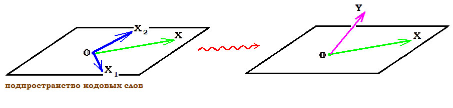
Если $ Xin mathbb V^{n}_{[k]} $ — кодовое слово, а $ Yin mathbb V^n $ — вектор, получившийся по прохождении этого слова по каналу, то $ Y-X $ называется вектором ошибок. Понятно, что при $ w(Y-X)=0 $ ошибки при передаче нет.
Предположим, что $ w(Y-X)=1 $, т.е. что при передаче произошла ошибка ровно в одном разряде кодового слова $ X_{} $. Попробуем ее обнаружить исходя из предположения, что кодовое слово выбиралось во множестве $ mathbb V^{n}_{[k]} $ линейного $ (n,k) $-кода, определенного в предыдущем пункте при какой-то проверочной матрице $ mathbf H $. Если для полученного вектора $ Y_{} $ выполняются все проверочные условия:
$$ Y cdot mathbf H^{top} = mathbb O_{1times k} , $$
(или, что то же $ Y in mathbb V^{n}_{[k]} $), то ошибка передачи считается не выявленной.
Для произвольного вектора $ Y in mathbb V^{n} $ вектор-строка
$$ S=Y cdot mathbf H^{top} in mathbb V^{k} $$
называется синдромом вектора Y. C точки зрения линейной алгебры его можно интерпретировать как показатель отхода вектора $ Y_{} $ от гиперплоскости, заданной системой однородных уравнений $ Xcdot mathbf H^{top}=mathbb O $.
Если синдром $ S_{} $ ненулевой: $ Y cdot mathbf H^{top} ne mathbb O_{1times k} $,
то полученный вектор $ Y_{} $ не принадлежит множеству $ mathbb V^{n}_{[k]} $ допустимых кодовых слов. Факт ошибки подтвержден. Изначально мы предположили, что произошла только одна ошибка, т.е.
$$ Y-X= {mathfrak e}_j = big(underbrace{0,dots,0,1}_{j},0,dots,0big) $$
при некотором $ jin {1,dots n} $. Тогда
$$ S= Y cdot mathbf H^{top} = (X+{mathfrak e}_j) cdot mathbf H^{top}=Xcdot mathbf H^{top}+
{mathfrak e}_j cdot mathbf H^{top}=
$$
$$
=mathbb O_{1times k} + mathbf H_{[j]}^{top} = mathbf H_{[j]}^{top}
$$
при $ mathbf H_{[j]} $ означающем $ j_{} $-й столбец проверочной матрицы $ mathbf H $. Таким образом получили соответствие
$$ {}_{} mathbf{HOMEP} mbox{ поврежденного бита} mathbf{=HOMEP} mbox{ столбца проверочной матрицы.} $$
И, следовательно, мы получили возможность обнаружить место повреждения — по факту совпадения синдрома со столбцом проверочной матрицы. К сожалению, реальность оказывается более сложной…![]()
П
Пример. В примере предыдущего пункта проверочная матрица была выбрана в виде
$$ mathbf H=
left( begin{array}{ccccc}
1 & 1 & 0 & 1 & 0 \
1 & 0 & 1 & 0 & 1
end{array}
right) .
$$
Если при передаче кодового слова $ (10011) $ произошла ошибка в первом бите, т.е. $ Y=(00011) $, то синдром
$$ S=Y cdot mathbf H^{top} = (11) $$
однозначно укажет на номер столбца матрицы $ mathbf H $. Если же ошибка произошла в четвертом бите, т.е. $ Y=(10001) $, то
$$ S=(10) , $$
но таких6) столбцов в матрице $ mathbf H $ два!
♦
Вывод. Для однозначного обнаружения места ошибки7) достаточно, чтобы все столбцы матрицы $ mathbf H $ были различными.
Столбцами этой матрицы являются транспонированные строки пространства $ mathbb V^{n-k} $.
Построение кода
Итак, исходя из соображений, завершающих предыдущий пункт, будем строить код, исправляющий одну ошибку, беря за стартовую точку именно матрицу $ mathbf H $. Выбираем ее произвольного порядка $ Mtimes N $ при $ {M,N} in mathbb N, M<N $ и вида
$$ mathbf H_{Mtimes N} = left[ tilde P mid E_M right] , $$
где матрица $ E_M $ — единичная порядка $ M_{} $, а матрица $ tilde P $ имеет порядок $ Mtimes (N-M) $, и столбцы ее должны быть различными, ненулевыми и отличаться от столбцов матрицы $ E_M $. По этой проверочной матрице — в соответствии со следствием к теореме $ 1 $ из
☞
ПУНКТА — строим порождающую матрицу:
$$ mathbf G_{(N-M)times N} = left[ E_{N-M} mid tilde P^{top} right] . $$
Строки матрицы $ mathbf G $ могут быть взяты в качестве базисных векторов подпространства кодовых слов.
П
Пример. Пусть $ M=2 $. Здесь имеем единственный вариант:
$$ mathbf H_{2times 3} = left( begin{array}{c|cc} 1 & 1 & 0 \ 1 & 0 & 1 end{array} right) , $$
поскольку в $ mathbb V^2 $ имеется лишь одна ненулевая строка, отличная от $ (10) $ и $ (01) $. Таким образом $ N=3 $ и
$$ mathbf G_{1times 3}=( 1, 1, 1 ) . $$
Следовательно, подпространство кодовых слов в $ mathbb V^3 $ является одномерным, и имеем всего два возможных кодовых слова: $ (000) $ и $ (111) $.
Пусть $ M=3 $. В $ mathbb V^3 $ имеется уже большой выбор строк, отличных от $ (100), (010), (001) $. Так, можно взять
$$
mathbf H_{3times 4} = left( begin{array}{c|ccc} 1 & 1 & 0 & 0 \ 1 & 0 & 1 & 0 \ 1 & 0 & 0 & 1 end{array} right) quad mbox{ или } quad
mathbf H_{3times 5} = left( begin{array}{cc|ccc} 1 & 0 & 1 & 0 & 0 \ 1 & 1 & 0 & 1 & 0 \ 0 & 1 & 0 & 0 & 1 end{array} right)
$$
$$
mbox{ или } quad
mathbf H_{3times 6} =
left( begin{array}{ccc|ccc} 1 & 0 & 1 & 1 & 0 & 0 \ 1 & 1 & 0 & 0 & 1 & 0 \ 0 & 1 & 1 & 0 & 0 & 1 end{array} right) quad mbox{ или } quad
mathbf H_{3times 7} =
left( begin{array}{cccc|ccc} 1 & 1 & 0 & 1 & 1 & 0 & 0 \ 1 & 1 & 1 & 0 & 0 & 1 & 0 \ 1 & 0 & 1 & 1 & 0 & 0 & 1 end{array} right) .
$$
Соответственно,
$$ mathbf G= (1, 1, 1, 1) quad quad mbox{ или } quad
mathbf G=
left( begin{array}{cc|ccc} 1 & 0 & 1 & 1 & 0 \ 0 & 1 & 0 & 1 & 1 end{array} right)
quad
$$
$$
mbox{ или } quad
mathbf G=
left( begin{array}{ccc|ccc} 1 & 0 & 0 & 1 & 1 & 0 \ 0 & 1 & 0 & 0 & 1 & 1 \ 0 & 0 & 1 & 1 & 0 & 1 end{array} right)
quad quad mbox{ или } quad
mathbf G=
left( begin{array}{cccc|ccc} 1 & 0 & 0 & 0 & 1 & 1 & 1 \ 0 & 1 & 0 & 0 & 1 & 1 & 0 \ 0 & 0 & 1 & 0 & 0 & 1 & 1 \ 0 & 0 & 0 & 1 & 1 & 0 & 1
end{array} right) .
$$
Кодовых векторов в соответствующих кодах будет $ 2^1,2^2,2^3,2^4 $. Любой из них способен исправить одну ошибку, полученную в ходе передачи.
♦
Если поставить задачу максимизации числа кодовых слов, то матрицу $ mathbf H $ следует выбирать самой широкой, т.е. делать $ N_{} $ максимально возможным. При фиксированном $ M_{} $ это достигается при выборе $ N=2^M-1 $. Тогда соответствующий линейный $ (n,k) $-код имеет значения параметров $ n=2^M-1,k=2^M-M-1 $, и именно он обычно и выбирается в качестве кода Хэмминга.
Найдем величину его кодового расстояния $ d_{} $. В соответствии с теоремой $ 3 $ из
☞
ПУНКТА, $ d>ell $, если любое подмножество из $ ell_{} $ столбцов матрицы $ mathbf H $ линейно независимо. Поскольку столбцы проверочной матрицы кода Хэмминга все различны, то любая пара из них линейно независима (свойство
3
☞
ЗДЕСЬ ). Следовательно, $ d>2 $. По теореме из
☞
ПУНКТА, получаем —
Если при передаче произошла ровно одна ошибка, то код Хэмминга способен ее исправить; если при передаче произошло ровно две ошибки, то код Хэмминга достоверно устанавливает лишь факт наличия ошибки.
Если попробовать исправить заглавие предыдущего пункта, исходя только из информации о структуре набора составляющих текст букв, то этой информации оказывается недостаточно: набор букв в правильном тексте будет таким же ![]()
П
Пример. Для проверочной матрицы $ (7,4) $-кода Хэмминга
$$
mathbf H_{3times 7} =
left( begin{array}{ccccccc} 1 & 1 & 0 & 1 & 1 & 0 & 0 \ 1 & 1 & 1 & 0 & 0 & 1 & 0 \ 1 & 0 & 1 & 1 & 0 & 0 & 1 end{array} right)
$$
вектор $ X=(0011110) $ является кодовым. Если при передаче произошла лишь одна ошибка и на выходе канала получили вектор $ Y=(1011110) $, то синдром этого вектора $ S=Y mathbf H^{top}=(111) $. Поскольку $ S^{top} $ совпадает с первым столбцом матрицы $ mathbf H $, то заключаем, что ошибка произошла в первом разряде. Тут же исправляем его на противоположный: $ X=Y+mathfrak e_1 $.
Если при передаче произошло две ошибки и на выходе канала получили вектор $ tilde Y=(1011010) $, то синдром этого вектора $ S=tilde Y mathbf H^{top}=(011) $. Поскольку синдром ненулевой, то факт наличия ошибки подтвержден. Однако корректно исправить ее — по аналогии с предыдущим — не удается. $ S^{top} $ совпадает с третьим столбцом матрицы $ mathbf H $, но в третьем разряде полученного вектора ошибки нет.
Наконец, если при передаче произошли три ошибки и на выходе канала получили вектор $ widehat Y=(1011011) $, то синдром этого вектора $ S=widehat Y mathbf H^{top}=(010) $. Наличие ошибки подтверждено, исправление невозможно. Если же — при передаче того же вектора $ X=(0011110) $ — получаем вектор
$ widehat Y_1=(1111111) $ (также с тремя ошибками), то его синдром оказывается нулевым: $ widehat Y_1 mathbf H^{top}=(000) $ и ошибка не обнаруживается.
♦
Проблема сравнения синдрома полученного вектора $ Y_{} $ со столбцами проверочной матрицы $ mathbf H $ с целью определения места ошибки — не такая тривиальная, особенно для больших $ n_{} $. Для упрощения этой процедуры воспользуемся следующим простым соображением. Размещение проверочных разрядов в конце кодового слова обусловлено лишь соображениями удобства изложения учебного материала. С точки зрения практической реализации, $ n-k $ проверочных разрядов можно разместить в любых местах кодового слова $ X_{} $ и даже «вразбивку», т.е. не подряд. Перестановке разрядов в кодовом слове будет соответствовать перестановка столбцов в матрице $ mathbf H $, при этом само множество столбцов остается неизменным — это транспонированные строки пространства $ mathbb V^{n-k} $ (ненулевые и различные). Рассмотрим $ (n,k) $-код Хэмминга при $ n=2^M-1,k=2^M-M-1, M ge 2 $. Тогда каждую ненулевую строку пространства $ mathbb V^{n-k}= mathbb V^M $ можно интерпретировать как двоичное представление числа из множества
$ {1,2,3,dots,2^M-1} $. Пусть
$$ j=underline{{mathfrak b}_1{mathfrak b}_2 dots {mathfrak b}_{M-1} {mathfrak b}_{M}}=
{mathfrak b}_1 times 2^{M-1}+{mathfrak b}_2 times 2^{M-2}+dots+{mathfrak b}_{M-1} times 2+ {mathfrak b}_{M} quad npu quad { {mathfrak b}_j}_{j=1}^Msubset {0,1} quad — $$
— двоичное представление числа $ j_{} $. Переупорядочим столбцы проверочной матрицы $ mathbf H $ так, чтобы
$$ mathbf H_{[j]}=left[ {mathfrak b}_1{mathfrak b}_2 dots {mathfrak b}_{M-1} {mathfrak b}_{M}right]^{top} , $$
т.е. чтобы $ j_{} $-й столбец содержал двоичное представление числа $ j_{} $. При таком упорядочении,
синдром произвольного вектора $ Y_{} $, отличающегося от кодового слова $ X_{} $ в единственном разряде, является двоичным представлением номера этого разряда:
$$ {bf mbox{СИНДРОМ }} (Y)=mathbf{HOMEP} (mbox{ошибочный разряд}) . $$
Осталось теперь выяснить какие разряды кодового слова содержат проверочные биты.
П
Пример. Для $ (7,4) $-кода Хэмминга матрицу $ mathbf H $, построенную в предыдущем примере, переупорядочим по столбцам; будем рассматривать ее в виде
$$
begin{array}{c}
left( begin{array}{ccccccc}
0 & 0 & 0 & 1 & 1 & 1 & 1 \
0 & 1 & 1 & 0 & 0 & 1 & 1 \
1 & 0 & 1 & 0 & 1 & 0 & 1
end{array} right) \
begin{array}{ccccccc}
uparrow & uparrow & uparrow & uparrow & uparrow & uparrow & uparrow \
scriptstyle 1 & scriptstyle 2 & scriptstyle 3 & scriptstyle 4 & scriptstyle 5 & scriptstyle 6 & scriptstyle 7
end{array}
end{array}
$$
Распишем проверочные соотношения $ Xmathbf H^{top}=mathbb O $ покомпонентно:
$$
left{
begin{array}{ccccccc}
& & & x_4&+x_5&+x_6&+x_7=0 \
&x_2&+x_3& & & +x_6&+x_7=0 \
x_1& & +x_3& & +x_5 & & +x_7=0
end{array} right. quad iff
$$
$$
iff quad
left{
begin{array}{ccccccc}
x_1& & +x_3& & +x_5 & & +x_7=0 \
&x_2&+x_3& & & +x_6&+x_7=0 \
& & & x_4&+x_5&+x_6&+x_7=0
end{array} right.
$$
Переписанные в последнем виде, эти уравнения представляют конечный пункт прямого хода метода Гаусса решения системы линейных уравнений, а именно — трапециевидную форму этой системы. Если бы мы поставили задачу поиска общего решения этой (однородной) системы и нахождения фундаментальной системы решений, то в качестве зависимых переменных однозначно бы выбрали $ x_1, x_2, x_4 $. Выпишем это общее решение8):
$$
x_1=x_3+x_5+x_7, x_2=x_3+x_6+x_7, x_4=x_5+x_6+x_7 .
$$
Это и есть проверочные соотношения, а проверочными разрядами кодового вектора являются $ 1_{} $-й, $ 2_{} $-й и $ 4_{} $-й.
Проверим правильность этих рассуждений. Придадим оставшимся разрядам произвольные значения, например:
$ x_3=1,x_5=1,x_6=0,x_7=1 $. Тогда $ x_1=1, x_2=0,x_4=0 $ и кодовый вектор $ X=(1010101) $. Пусть на выходе из канала он превратился в $ Y=(1000101) $. Синдром этого вектора $ Ymathbf H^{top}=(011) $ — это двоичное представление числа $ 3_{} $. И ведь действительно: ошибка — в третьем разряде!
♦
Алгоритм построения (n,k)-кода Хэмминга
для $ n=2^M-1,k=2^M-M-1, M ge 2 $.
1.
Строится матрица $ mathbf H $ порядка $ M times (2^M-1) $ из столбцов, представляющих двоичные представления чисел $ {1,2,3,dots,2^M-1} $ (младшие разряды — внизу).
2.
Проверочные разряды имеют номера, равные степеням двойки: $ 1,2,2^2,dots,2^{M-1} $.
3.
Проверочные соотношения получаются из матричного представления $ Xmathbf H^{top}=mathbb O $ выражением проверочных разрядов через информационные.
Можно немного улучшить код Хэмминга, увеличив кодовое расстояние до $ 4_{} $.
?
Является ли $ 8_{} $-мибитный код Адамара из примера
☞
ПУНКТА линейным кодом?
.
Источники
[1]. Питерсон У., Уэлдон Э. Коды, исправляющие ошибки. М.Мир. 1976.
[2]. Марков А.А. Введение в теорию кодирования. М.Наука. 1982
| Binary Hamming codes | |
|---|---|

The Hamming(7,4) code (with r = 3) |
|
| Named after | Richard W. Hamming |
| Classification | |
| Type | Linear block code |
| Block length | 2r − 1 where r ≥ 2 |
| Message length | 2r − r − 1 |
| Rate | 1 − r/(2r − 1) |
| Distance | 3 |
| Alphabet size | 2 |
| Notation | [2r − 1, 2r − r − 1, 3]2-code |
| Properties | |
| perfect code | |
|
In computer science and telecommunication, Hamming codes are a family of linear error-correcting codes. Hamming codes can detect one-bit and two-bit errors, or correct one-bit errors without detection of uncorrected errors. By contrast, the simple parity code cannot correct errors, and can detect only an odd number of bits in error. Hamming codes are perfect codes, that is, they achieve the highest possible rate for codes with their block length and minimum distance of three.[1]
Richard W. Hamming invented Hamming codes in 1950 as a way of automatically correcting errors introduced by punched card readers. In his original paper, Hamming elaborated his general idea, but specifically focused on the Hamming(7,4) code which adds three parity bits to four bits of data.[2]
In mathematical terms, Hamming codes are a class of binary linear code. For each integer r ≥ 2 there is a code-word with block length n = 2r − 1 and message length k = 2r − r − 1. Hence the rate of Hamming codes is R = k / n = 1 − r / (2r − 1), which is the highest possible for codes with minimum distance of three (i.e., the minimal number of bit changes needed to go from any code word to any other code word is three) and block length 2r − 1. The parity-check matrix of a Hamming code is constructed by listing all columns of length r that are non-zero, which means that the dual code of the Hamming code is the shortened Hadamard code. The parity-check matrix has the property that any two columns are pairwise linearly independent.
Due to the limited redundancy that Hamming codes add to the data, they can only detect and correct errors when the error rate is low. This is the case in computer memory (usually RAM), where bit errors are extremely rare and Hamming codes are widely used, and a RAM with this correction system is a ECC RAM (ECC memory). In this context, an extended Hamming code having one extra parity bit is often used. Extended Hamming codes achieve a Hamming distance of four, which allows the decoder to distinguish between when at most one one-bit error occurs and when any two-bit errors occur. In this sense, extended Hamming codes are single-error correcting and double-error detecting, abbreviated as SECDED.
History[edit]
Richard Hamming, the inventor of Hamming codes, worked at Bell Labs in the late 1940s on the Bell Model V computer, an electromechanical relay-based machine with cycle times in seconds. Input was fed in on punched paper tape, seven-eighths of an inch wide, which had up to six holes per row. During weekdays, when errors in the relays were detected, the machine would stop and flash lights so that the operators could correct the problem. During after-hours periods and on weekends, when there were no operators, the machine simply moved on to the next job.
Hamming worked on weekends, and grew increasingly frustrated with having to restart his programs from scratch due to detected errors. In a taped interview, Hamming said, «And so I said, ‘Damn it, if the machine can detect an error, why can’t it locate the position of the error and correct it?'».[3] Over the next few years, he worked on the problem of error-correction, developing an increasingly powerful array of algorithms. In 1950, he published what is now known as Hamming code, which remains in use today in applications such as ECC memory.
Codes predating Hamming[edit]
A number of simple error-detecting codes were used before Hamming codes, but none were as effective as Hamming codes in the same overhead of space.
Parity[edit]
Parity adds a single bit that indicates whether the number of ones (bit-positions with values of one) in the preceding data was even or odd. If an odd number of bits is changed in transmission, the message will change parity and the error can be detected at this point; however, the bit that changed may have been the parity bit itself. The most common convention is that a parity value of one indicates that there is an odd number of ones in the data, and a parity value of zero indicates that there is an even number of ones. If the number of bits changed is even, the check bit will be valid and the error will not be detected.
Moreover, parity does not indicate which bit contained the error, even when it can detect it. The data must be discarded entirely and re-transmitted from scratch. On a noisy transmission medium, a successful transmission could take a long time or may never occur. However, while the quality of parity checking is poor, since it uses only a single bit, this method results in the least overhead.
Two-out-of-five code[edit]
A two-out-of-five code is an encoding scheme which uses five bits consisting of exactly three 0s and two 1s. This provides ten possible combinations, enough to represent the digits 0–9. This scheme can detect all single bit-errors, all odd numbered bit-errors and some even numbered bit-errors (for example the flipping of both 1-bits). However it still cannot correct any of these errors.
Repetition[edit]
Another code in use at the time repeated every data bit multiple times in order to ensure that it was sent correctly. For instance, if the data bit to be sent is a 1, an n = 3 repetition code will send 111. If the three bits received are not identical, an error occurred during transmission. If the channel is clean enough, most of the time only one bit will change in each triple. Therefore, 001, 010, and 100 each correspond to a 0 bit, while 110, 101, and 011 correspond to a 1 bit, with the greater quantity of digits that are the same (‘0’ or a ‘1’) indicating what the data bit should be. A code with this ability to reconstruct the original message in the presence of errors is known as an error-correcting code. This triple repetition code is a Hamming code with m = 2, since there are two parity bits, and 22 − 2 − 1 = 1 data bit.
Such codes cannot correctly repair all errors, however. In our example, if the channel flips two bits and the receiver gets 001, the system will detect the error, but conclude that the original bit is 0, which is incorrect. If we increase the size of the bit string to four, we can detect all two-bit errors but cannot correct them (the quantity of parity bits is even); at five bits, we can both detect and correct all two-bit errors, but not all three-bit errors.
Moreover, increasing the size of the parity bit string is inefficient, reducing throughput by three times in our original case, and the efficiency drops drastically as we increase the number of times each bit is duplicated in order to detect and correct more errors.
Description[edit]
If more error-correcting bits are included with a message, and if those bits can be arranged such that different incorrect bits produce different error results, then bad bits could be identified. In a seven-bit message, there are seven possible single bit errors, so three error control bits could potentially specify not only that an error occurred but also which bit caused the error.
Hamming studied the existing coding schemes, including two-of-five, and generalized their concepts. To start with, he developed a nomenclature to describe the system, including the number of data bits and error-correction bits in a block. For instance, parity includes a single bit for any data word, so assuming ASCII words with seven bits, Hamming described this as an (8,7) code, with eight bits in total, of which seven are data. The repetition example would be (3,1), following the same logic. The code rate is the second number divided by the first, for our repetition example, 1/3.
Hamming also noticed the problems with flipping two or more bits, and described this as the «distance» (it is now called the Hamming distance, after him). Parity has a distance of 2, so one bit flip can be detected but not corrected, and any two bit flips will be invisible. The (3,1) repetition has a distance of 3, as three bits need to be flipped in the same triple to obtain another code word with no visible errors. It can correct one-bit errors or it can detect — but not correct — two-bit errors. A (4,1) repetition (each bit is repeated four times) has a distance of 4, so flipping three bits can be detected, but not corrected. When three bits flip in the same group there can be situations where attempting to correct will produce the wrong code word. In general, a code with distance k can detect but not correct k − 1 errors.
Hamming was interested in two problems at once: increasing the distance as much as possible, while at the same time increasing the code rate as much as possible. During the 1940s he developed several encoding schemes that were dramatic improvements on existing codes. The key to all of his systems was to have the parity bits overlap, such that they managed to check each other as well as the data.
General algorithm[edit]
The following general algorithm generates a single-error correcting (SEC) code for any number of bits. The main idea is to choose the error-correcting bits such that the index-XOR (the XOR of all the bit positions containing a 1) is 0. We use positions 1, 10, 100, etc. (in binary) as the error-correcting bits, which guarantees it is possible to set the error-correcting bits so that the index-XOR of the whole message is 0. If the receiver receives a string with index-XOR 0, they can conclude there were no corruptions, and otherwise, the index-XOR indicates the index of the corrupted bit.
An algorithm can be deduced from the following description:
- Number the bits starting from 1: bit 1, 2, 3, 4, 5, 6, 7, etc.
- Write the bit numbers in binary: 1, 10, 11, 100, 101, 110, 111, etc.
- All bit positions that are powers of two (have a single 1 bit in the binary form of their position) are parity bits: 1, 2, 4, 8, etc. (1, 10, 100, 1000)
- All other bit positions, with two or more 1 bits in the binary form of their position, are data bits.
- Each data bit is included in a unique set of 2 or more parity bits, as determined by the binary form of its bit position.
- Parity bit 1 covers all bit positions which have the least significant bit set: bit 1 (the parity bit itself), 3, 5, 7, 9, etc.
- Parity bit 2 covers all bit positions which have the second least significant bit set: bits 2-3, 6-7, 10-11, etc.
- Parity bit 4 covers all bit positions which have the third least significant bit set: bits 4–7, 12–15, 20–23, etc.
- Parity bit 8 covers all bit positions which have the fourth least significant bit set: bits 8–15, 24–31, 40–47, etc.
- In general each parity bit covers all bits where the bitwise AND of the parity position and the bit position is non-zero.
If a byte of data to be encoded is 10011010, then the data word (using _ to represent the parity bits) would be __1_001_1010, and the code word is 011100101010.
The choice of the parity, even or odd, is irrelevant but the same choice must be used for both encoding and decoding.
This general rule can be shown visually:
-
Bit position 1 2 3 4 5 6 7 8 9 10 11 12 13 14 15 16 17 18 19 20 … Encoded data bits p1 p2 d1 p4 d2 d3 d4 p8 d5 d6 d7 d8 d9 d10 d11 p16 d12 d13 d14 d15 Parity
bit
coveragep1 
p2 p4
p8 p16
Shown are only 20 encoded bits (5 parity, 15 data) but the pattern continues indefinitely. The key thing about Hamming Codes that can be seen from visual inspection is that any given bit is included in a unique set of parity bits. To check for errors, check all of the parity bits. The pattern of errors, called the error syndrome, identifies the bit in error. If all parity bits are correct, there is no error. Otherwise, the sum of the positions of the erroneous parity bits identifies the erroneous bit. For example, if the parity bits in positions 1, 2 and 8 indicate an error, then bit 1+2+8=11 is in error. If only one parity bit indicates an error, the parity bit itself is in error.
With m parity bits, bits from 1 up to 

| Parity bits | Total bits | Data bits | Name | Rate |
|---|---|---|---|---|
| 2 | 3 | 1 | Hamming(3,1) (Triple repetition code) |
1/3 ≈ 0.333 |
| 3 | 7 | 4 | Hamming(7,4) | 4/7 ≈ 0.571 |
| 4 | 15 | 11 | Hamming(15,11) | 11/15 ≈ 0.733 |
| 5 | 31 | 26 | Hamming(31,26) | 26/31 ≈ 0.839 |
| 6 | 63 | 57 | Hamming(63,57) | 57/63 ≈ 0.905 |
| 7 | 127 | 120 | Hamming(127,120) | 120/127 ≈ 0.945 |
| 8 | 255 | 247 | Hamming(255,247) | 247/255 ≈ 0.969 |
| … | ||||
| m |  |
 |
Hamming |

|
Hamming codes with additional parity (SECDED)[edit]
Hamming codes have a minimum distance of 3, which means that the decoder can detect and correct a single error, but it cannot distinguish a double bit error of some codeword from a single bit error of a different codeword. Thus, some double-bit errors will be incorrectly decoded as if they were single bit errors and therefore go undetected, unless no correction is attempted.
To remedy this shortcoming, Hamming codes can be extended by an extra parity bit. This way, it is possible to increase the minimum distance of the Hamming code to 4, which allows the decoder to distinguish between single bit errors and two-bit errors. Thus the decoder can detect and correct a single error and at the same time detect (but not correct) a double error.
If the decoder does not attempt to correct errors, it can reliably detect triple bit errors. If the decoder does correct errors, some triple errors will be mistaken for single errors and «corrected» to the wrong value. Error correction is therefore a trade-off between certainty (the ability to reliably detect triple bit errors) and resiliency (the ability to keep functioning in the face of single bit errors).
This extended Hamming code was popular in computer memory systems, starting with IBM 7030 Stretch in 1961,[4] where it is known as SECDED (or SEC-DED, abbreviated from single error correction, double error detection).[5] Server computers in 21st century, while typically keeping the SECDED level of protection, no longer use the Hamming’s method, relying instead on the designs with longer codewords (128 to 256 bits of data) and modified balanced parity-check trees.[4] The (72,64) Hamming code is still popular in some hardware designs, including Xilinx FPGA families.[4]
[7,4] Hamming code[edit]

Graphical depiction of the four data bits and three parity bits and which parity bits apply to which data bits
In 1950, Hamming introduced the [7,4] Hamming code. It encodes four data bits into seven bits by adding three parity bits. It can detect and correct single-bit errors. With the addition of an overall parity bit, it can also detect (but not correct) double-bit errors.
Construction of G and H[edit]
The matrix

and 
This is the construction of G and H in standard (or systematic) form. Regardless of form, G and H for linear block codes must satisfy

Since [7, 4, 3] = [n, k, d] = [2m − 1, 2m − 1 − m, 3]. The parity-check matrix H of a Hamming code is constructed by listing all columns of length m that are pair-wise independent.
Thus H is a matrix whose left side is all of the nonzero n-tuples where order of the n-tuples in the columns of matrix does not matter. The right hand side is just the (n − k)-identity matrix.
So G can be obtained from H by taking the transpose of the left hand side of H with the identity k-identity matrix on the left hand side of G.
The code generator matrix 


and

Finally, these matrices can be mutated into equivalent non-systematic codes by the following operations:[6]
- Column permutations (swapping columns)
- Elementary row operations (replacing a row with a linear combination of rows)
Encoding[edit]
- Example
From the above matrix we have 2k = 24 = 16 codewords.
Let 
![{displaystyle {vec {a}}=[a_{1},a_{2},a_{3},a_{4}],quad a_{i}in {0,1}}](https://wikimedia.org/api/rest_v1/media/math/render/svg/898ddf319567d4af0acecf5c7fd450f5f466e28b)


For example, let ![{displaystyle {vec {a}}=[1,0,1,1]}](https://wikimedia.org/api/rest_v1/media/math/render/svg/e838e2ec81e9fe6223596b61f747b195d3d338fb)


[7,4] Hamming code with an additional parity bit[edit]

The same [7,4] example from above with an extra parity bit. This diagram is not meant to correspond to the matrix H for this example.
The [7,4] Hamming code can easily be extended to an [8,4] code by adding an extra parity bit on top of the (7,4) encoded word (see Hamming(7,4)).
This can be summed up with the revised matrices:

and

Note that H is not in standard form. To obtain G, elementary row operations can be used to obtain an equivalent matrix to H in systematic form:

For example, the first row in this matrix is the sum of the second and third rows of H in non-systematic form. Using the systematic construction for Hamming codes from above, the matrix A is apparent and the systematic form of G is written as

The non-systematic form of G can be row reduced (using elementary row operations) to match this matrix.
The addition of the fourth row effectively computes the sum of all the codeword bits (data and parity) as the fourth parity bit.
For example, 1011 is encoded (using the non-systematic form of G at the start of this section) into 01100110 where blue digits are data; red digits are parity bits from the [7,4] Hamming code; and the green digit is the parity bit added by the [8,4] code.
The green digit makes the parity of the [7,4] codewords even.
Finally, it can be shown that the minimum distance has increased from 3, in the [7,4] code, to 4 in the [8,4] code. Therefore, the code can be defined as [8,4] Hamming code.
To decode the [8,4] Hamming code, first check the parity bit. If the parity bit indicates an error, single error correction (the [7,4] Hamming code) will indicate the error location, with «no error» indicating the parity bit. If the parity bit is correct, then single error correction will indicate the (bitwise) exclusive-or of two error locations. If the locations are equal («no error») then a double bit error either has not occurred, or has cancelled itself out. Otherwise, a double bit error has occurred.
See also[edit]
- Coding theory
- Golay code
- Reed–Muller code
- Reed–Solomon error correction
- Turbo code
- Low-density parity-check code
- Hamming bound
- Hamming distance
Notes[edit]
- ^ See Lemma 12 of
- ^ Hamming (1950), pp. 153–154.
- ^ Thompson, Thomas M. (1983), From Error-Correcting Codes through Sphere Packings to Simple Groups, The Carus Mathematical Monographs (#21), Mathematical Association of America, pp. 16–17, ISBN 0-88385-023-0
- ^ a b c Kythe & Kythe 2017, p. 115.
- ^ Kythe & Kythe 2017, p. 95.
- ^ a b Moon T. Error correction coding: Mathematical Methods and
Algorithms. John Wiley and Sons, 2005.(Cap. 3) ISBN 978-0-471-64800-0
References[edit]
- Hamming, Richard Wesley (1950). «Error detecting and error correcting codes» (PDF). Bell System Technical Journal. 29 (2): 147–160. doi:10.1002/j.1538-7305.1950.tb00463.x. S2CID 61141773. Archived (PDF) from the original on 2022-10-09.
- Moon, Todd K. (2005). Error Correction Coding. New Jersey: John Wiley & Sons. ISBN 978-0-471-64800-0.
- MacKay, David J.C. (September 2003). Information Theory, Inference and Learning Algorithms. Cambridge: Cambridge University Press. ISBN 0-521-64298-1.
- D.K. Bhattacharryya, S. Nandi. «An efficient class of SEC-DED-AUED codes». 1997 International Symposium on Parallel Architectures, Algorithms and Networks (ISPAN ’97). pp. 410–415. doi:10.1109/ISPAN.1997.645128.
- «Mathematical Challenge April 2013 Error-correcting codes» (PDF). swissQuant Group Leadership Team. April 2013. Archived (PDF) from the original on 2017-09-12.
- Kythe, Dave K.; Kythe, Prem K. (28 July 2017). «Extended Hamming Codes». Algebraic and Stochastic Coding Theory. CRC Press. pp. 95–116. ISBN 978-1-351-83245-8.
External links[edit]
- Visual Explanation of Hamming Codes
- CGI script for calculating Hamming distances (from R. Tervo, UNB, Canada)
- Tool for calculating Hamming code
| Binary Hamming codes | |
|---|---|
|
The Hamming(7,4) code (with r = 3) |
|
| Named after | Richard W. Hamming |
| Classification | |
| Type | Linear block code |
| Block length | 2r − 1 where r ≥ 2 |
| Message length | 2r − r − 1 |
| Rate | 1 − r/(2r − 1) |
| Distance | 3 |
| Alphabet size | 2 |
| Notation | [2r − 1, 2r − r − 1, 3]2-code |
| Properties | |
| perfect code | |
|
In computer science and telecommunication, Hamming codes are a family of linear error-correcting codes. Hamming codes can detect one-bit and two-bit errors, or correct one-bit errors without detection of uncorrected errors. By contrast, the simple parity code cannot correct errors, and can detect only an odd number of bits in error. Hamming codes are perfect codes, that is, they achieve the highest possible rate for codes with their block length and minimum distance of three.[1]
Richard W. Hamming invented Hamming codes in 1950 as a way of automatically correcting errors introduced by punched card readers. In his original paper, Hamming elaborated his general idea, but specifically focused on the Hamming(7,4) code which adds three parity bits to four bits of data.[2]
In mathematical terms, Hamming codes are a class of binary linear code. For each integer r ≥ 2 there is a code-word with block length n = 2r − 1 and message length k = 2r − r − 1. Hence the rate of Hamming codes is R = k / n = 1 − r / (2r − 1), which is the highest possible for codes with minimum distance of three (i.e., the minimal number of bit changes needed to go from any code word to any other code word is three) and block length 2r − 1. The parity-check matrix of a Hamming code is constructed by listing all columns of length r that are non-zero, which means that the dual code of the Hamming code is the shortened Hadamard code. The parity-check matrix has the property that any two columns are pairwise linearly independent.
Due to the limited redundancy that Hamming codes add to the data, they can only detect and correct errors when the error rate is low. This is the case in computer memory (usually RAM), where bit errors are extremely rare and Hamming codes are widely used, and a RAM with this correction system is a ECC RAM (ECC memory). In this context, an extended Hamming code having one extra parity bit is often used. Extended Hamming codes achieve a Hamming distance of four, which allows the decoder to distinguish between when at most one one-bit error occurs and when any two-bit errors occur. In this sense, extended Hamming codes are single-error correcting and double-error detecting, abbreviated as SECDED.
History[edit]
Richard Hamming, the inventor of Hamming codes, worked at Bell Labs in the late 1940s on the Bell Model V computer, an electromechanical relay-based machine with cycle times in seconds. Input was fed in on punched paper tape, seven-eighths of an inch wide, which had up to six holes per row. During weekdays, when errors in the relays were detected, the machine would stop and flash lights so that the operators could correct the problem. During after-hours periods and on weekends, when there were no operators, the machine simply moved on to the next job.
Hamming worked on weekends, and grew increasingly frustrated with having to restart his programs from scratch due to detected errors. In a taped interview, Hamming said, «And so I said, ‘Damn it, if the machine can detect an error, why can’t it locate the position of the error and correct it?'».[3] Over the next few years, he worked on the problem of error-correction, developing an increasingly powerful array of algorithms. In 1950, he published what is now known as Hamming code, which remains in use today in applications such as ECC memory.
Codes predating Hamming[edit]
A number of simple error-detecting codes were used before Hamming codes, but none were as effective as Hamming codes in the same overhead of space.
Parity[edit]
Parity adds a single bit that indicates whether the number of ones (bit-positions with values of one) in the preceding data was even or odd. If an odd number of bits is changed in transmission, the message will change parity and the error can be detected at this point; however, the bit that changed may have been the parity bit itself. The most common convention is that a parity value of one indicates that there is an odd number of ones in the data, and a parity value of zero indicates that there is an even number of ones. If the number of bits changed is even, the check bit will be valid and the error will not be detected.
Moreover, parity does not indicate which bit contained the error, even when it can detect it. The data must be discarded entirely and re-transmitted from scratch. On a noisy transmission medium, a successful transmission could take a long time or may never occur. However, while the quality of parity checking is poor, since it uses only a single bit, this method results in the least overhead.
Two-out-of-five code[edit]
A two-out-of-five code is an encoding scheme which uses five bits consisting of exactly three 0s and two 1s. This provides ten possible combinations, enough to represent the digits 0–9. This scheme can detect all single bit-errors, all odd numbered bit-errors and some even numbered bit-errors (for example the flipping of both 1-bits). However it still cannot correct any of these errors.
Repetition[edit]
Another code in use at the time repeated every data bit multiple times in order to ensure that it was sent correctly. For instance, if the data bit to be sent is a 1, an n = 3 repetition code will send 111. If the three bits received are not identical, an error occurred during transmission. If the channel is clean enough, most of the time only one bit will change in each triple. Therefore, 001, 010, and 100 each correspond to a 0 bit, while 110, 101, and 011 correspond to a 1 bit, with the greater quantity of digits that are the same (‘0’ or a ‘1’) indicating what the data bit should be. A code with this ability to reconstruct the original message in the presence of errors is known as an error-correcting code. This triple repetition code is a Hamming code with m = 2, since there are two parity bits, and 22 − 2 − 1 = 1 data bit.
Such codes cannot correctly repair all errors, however. In our example, if the channel flips two bits and the receiver gets 001, the system will detect the error, but conclude that the original bit is 0, which is incorrect. If we increase the size of the bit string to four, we can detect all two-bit errors but cannot correct them (the quantity of parity bits is even); at five bits, we can both detect and correct all two-bit errors, but not all three-bit errors.
Moreover, increasing the size of the parity bit string is inefficient, reducing throughput by three times in our original case, and the efficiency drops drastically as we increase the number of times each bit is duplicated in order to detect and correct more errors.
Description[edit]
If more error-correcting bits are included with a message, and if those bits can be arranged such that different incorrect bits produce different error results, then bad bits could be identified. In a seven-bit message, there are seven possible single bit errors, so three error control bits could potentially specify not only that an error occurred but also which bit caused the error.
Hamming studied the existing coding schemes, including two-of-five, and generalized their concepts. To start with, he developed a nomenclature to describe the system, including the number of data bits and error-correction bits in a block. For instance, parity includes a single bit for any data word, so assuming ASCII words with seven bits, Hamming described this as an (8,7) code, with eight bits in total, of which seven are data. The repetition example would be (3,1), following the same logic. The code rate is the second number divided by the first, for our repetition example, 1/3.
Hamming also noticed the problems with flipping two or more bits, and described this as the «distance» (it is now called the Hamming distance, after him). Parity has a distance of 2, so one bit flip can be detected but not corrected, and any two bit flips will be invisible. The (3,1) repetition has a distance of 3, as three bits need to be flipped in the same triple to obtain another code word with no visible errors. It can correct one-bit errors or it can detect — but not correct — two-bit errors. A (4,1) repetition (each bit is repeated four times) has a distance of 4, so flipping three bits can be detected, but not corrected. When three bits flip in the same group there can be situations where attempting to correct will produce the wrong code word. In general, a code with distance k can detect but not correct k − 1 errors.
Hamming was interested in two problems at once: increasing the distance as much as possible, while at the same time increasing the code rate as much as possible. During the 1940s he developed several encoding schemes that were dramatic improvements on existing codes. The key to all of his systems was to have the parity bits overlap, such that they managed to check each other as well as the data.
General algorithm[edit]
The following general algorithm generates a single-error correcting (SEC) code for any number of bits. The main idea is to choose the error-correcting bits such that the index-XOR (the XOR of all the bit positions containing a 1) is 0. We use positions 1, 10, 100, etc. (in binary) as the error-correcting bits, which guarantees it is possible to set the error-correcting bits so that the index-XOR of the whole message is 0. If the receiver receives a string with index-XOR 0, they can conclude there were no corruptions, and otherwise, the index-XOR indicates the index of the corrupted bit.
An algorithm can be deduced from the following description:
- Number the bits starting from 1: bit 1, 2, 3, 4, 5, 6, 7, etc.
- Write the bit numbers in binary: 1, 10, 11, 100, 101, 110, 111, etc.
- All bit positions that are powers of two (have a single 1 bit in the binary form of their position) are parity bits: 1, 2, 4, 8, etc. (1, 10, 100, 1000)
- All other bit positions, with two or more 1 bits in the binary form of their position, are data bits.
- Each data bit is included in a unique set of 2 or more parity bits, as determined by the binary form of its bit position.
- Parity bit 1 covers all bit positions which have the least significant bit set: bit 1 (the parity bit itself), 3, 5, 7, 9, etc.
- Parity bit 2 covers all bit positions which have the second least significant bit set: bits 2-3, 6-7, 10-11, etc.
- Parity bit 4 covers all bit positions which have the third least significant bit set: bits 4–7, 12–15, 20–23, etc.
- Parity bit 8 covers all bit positions which have the fourth least significant bit set: bits 8–15, 24–31, 40–47, etc.
- In general each parity bit covers all bits where the bitwise AND of the parity position and the bit position is non-zero.
If a byte of data to be encoded is 10011010, then the data word (using _ to represent the parity bits) would be __1_001_1010, and the code word is 011100101010.
The choice of the parity, even or odd, is irrelevant but the same choice must be used for both encoding and decoding.
This general rule can be shown visually:
-
Bit position 1 2 3 4 5 6 7 8 9 10 11 12 13 14 15 16 17 18 19 20 … Encoded data bits p1 p2 d1 p4 d2 d3 d4 p8 d5 d6 d7 d8 d9 d10 d11 p16 d12 d13 d14 d15 Parity
bit
coveragep1 p2 p4
p8 p16
Shown are only 20 encoded bits (5 parity, 15 data) but the pattern continues indefinitely. The key thing about Hamming Codes that can be seen from visual inspection is that any given bit is included in a unique set of parity bits. To check for errors, check all of the parity bits. The pattern of errors, called the error syndrome, identifies the bit in error. If all parity bits are correct, there is no error. Otherwise, the sum of the positions of the erroneous parity bits identifies the erroneous bit. For example, if the parity bits in positions 1, 2 and 8 indicate an error, then bit 1+2+8=11 is in error. If only one parity bit indicates an error, the parity bit itself is in error.
With m parity bits, bits from 1 up to
| Parity bits | Total bits | Data bits | Name | Rate |
|---|---|---|---|---|
| 2 | 3 | 1 | Hamming(3,1) (Triple repetition code) |
1/3 ≈ 0.333 |
| 3 | 7 | 4 | Hamming(7,4) | 4/7 ≈ 0.571 |
| 4 | 15 | 11 | Hamming(15,11) | 11/15 ≈ 0.733 |
| 5 | 31 | 26 | Hamming(31,26) | 26/31 ≈ 0.839 |
| 6 | 63 | 57 | Hamming(63,57) | 57/63 ≈ 0.905 |
| 7 | 127 | 120 | Hamming(127,120) | 120/127 ≈ 0.945 |
| 8 | 255 | 247 | Hamming(255,247) | 247/255 ≈ 0.969 |
| … | ||||
| m | |
|
Hamming |
|
Hamming codes with additional parity (SECDED)[edit]
Hamming codes have a minimum distance of 3, which means that the decoder can detect and correct a single error, but it cannot distinguish a double bit error of some codeword from a single bit error of a different codeword. Thus, some double-bit errors will be incorrectly decoded as if they were single bit errors and therefore go undetected, unless no correction is attempted.
To remedy this shortcoming, Hamming codes can be extended by an extra parity bit. This way, it is possible to increase the minimum distance of the Hamming code to 4, which allows the decoder to distinguish between single bit errors and two-bit errors. Thus the decoder can detect and correct a single error and at the same time detect (but not correct) a double error.
If the decoder does not attempt to correct errors, it can reliably detect triple bit errors. If the decoder does correct errors, some triple errors will be mistaken for single errors and «corrected» to the wrong value. Error correction is therefore a trade-off between certainty (the ability to reliably detect triple bit errors) and resiliency (the ability to keep functioning in the face of single bit errors).
This extended Hamming code was popular in computer memory systems, starting with IBM 7030 Stretch in 1961,[4] where it is known as SECDED (or SEC-DED, abbreviated from single error correction, double error detection).[5] Server computers in 21st century, while typically keeping the SECDED level of protection, no longer use the Hamming’s method, relying instead on the designs with longer codewords (128 to 256 bits of data) and modified balanced parity-check trees.[4] The (72,64) Hamming code is still popular in some hardware designs, including Xilinx FPGA families.[4]
[7,4] Hamming code[edit]
Graphical depiction of the four data bits and three parity bits and which parity bits apply to which data bits
In 1950, Hamming introduced the [7,4] Hamming code. It encodes four data bits into seven bits by adding three parity bits. It can detect and correct single-bit errors. With the addition of an overall parity bit, it can also detect (but not correct) double-bit errors.
Construction of G and H[edit]
The matrix
and
This is the construction of G and H in standard (or systematic) form. Regardless of form, G and H for linear block codes must satisfy
Since [7, 4, 3] = [n, k, d] = [2m − 1, 2m − 1 − m, 3]. The parity-check matrix H of a Hamming code is constructed by listing all columns of length m that are pair-wise independent.
Thus H is a matrix whose left side is all of the nonzero n-tuples where order of the n-tuples in the columns of matrix does not matter. The right hand side is just the (n − k)-identity matrix.
So G can be obtained from H by taking the transpose of the left hand side of H with the identity k-identity matrix on the left hand side of G.
The code generator matrix
and
Finally, these matrices can be mutated into equivalent non-systematic codes by the following operations:[6]
- Column permutations (swapping columns)
- Elementary row operations (replacing a row with a linear combination of rows)
Encoding[edit]
- Example
From the above matrix we have 2k = 24 = 16 codewords.
Let
For example, let
[7,4] Hamming code with an additional parity bit[edit]
The same [7,4] example from above with an extra parity bit. This diagram is not meant to correspond to the matrix H for this example.
The [7,4] Hamming code can easily be extended to an [8,4] code by adding an extra parity bit on top of the (7,4) encoded word (see Hamming(7,4)).
This can be summed up with the revised matrices:
and
Note that H is not in standard form. To obtain G, elementary row operations can be used to obtain an equivalent matrix to H in systematic form:
For example, the first row in this matrix is the sum of the second and third rows of H in non-systematic form. Using the systematic construction for Hamming codes from above, the matrix A is apparent and the systematic form of G is written as
The non-systematic form of G can be row reduced (using elementary row operations) to match this matrix.
The addition of the fourth row effectively computes the sum of all the codeword bits (data and parity) as the fourth parity bit.
For example, 1011 is encoded (using the non-systematic form of G at the start of this section) into 01100110 where blue digits are data; red digits are parity bits from the [7,4] Hamming code; and the green digit is the parity bit added by the [8,4] code.
The green digit makes the parity of the [7,4] codewords even.
Finally, it can be shown that the minimum distance has increased from 3, in the [7,4] code, to 4 in the [8,4] code. Therefore, the code can be defined as [8,4] Hamming code.
To decode the [8,4] Hamming code, first check the parity bit. If the parity bit indicates an error, single error correction (the [7,4] Hamming code) will indicate the error location, with «no error» indicating the parity bit. If the parity bit is correct, then single error correction will indicate the (bitwise) exclusive-or of two error locations. If the locations are equal («no error») then a double bit error either has not occurred, or has cancelled itself out. Otherwise, a double bit error has occurred.
See also[edit]
- Coding theory
- Golay code
- Reed–Muller code
- Reed–Solomon error correction
- Turbo code
- Low-density parity-check code
- Hamming bound
- Hamming distance
Notes[edit]
- ^ See Lemma 12 of
- ^ Hamming (1950), pp. 153–154.
- ^ Thompson, Thomas M. (1983), From Error-Correcting Codes through Sphere Packings to Simple Groups, The Carus Mathematical Monographs (#21), Mathematical Association of America, pp. 16–17, ISBN 0-88385-023-0
- ^ a b c Kythe & Kythe 2017, p. 115.
- ^ Kythe & Kythe 2017, p. 95.
- ^ a b Moon T. Error correction coding: Mathematical Methods and
Algorithms. John Wiley and Sons, 2005.(Cap. 3) ISBN 978-0-471-64800-0
References[edit]
- Hamming, Richard Wesley (1950). «Error detecting and error correcting codes» (PDF). Bell System Technical Journal. 29 (2): 147–160. doi:10.1002/j.1538-7305.1950.tb00463.x. S2CID 61141773. Archived (PDF) from the original on 2022-10-09.
- Moon, Todd K. (2005). Error Correction Coding. New Jersey: John Wiley & Sons. ISBN 978-0-471-64800-0.
- MacKay, David J.C. (September 2003). Information Theory, Inference and Learning Algorithms. Cambridge: Cambridge University Press. ISBN 0-521-64298-1.
- D.K. Bhattacharryya, S. Nandi. «An efficient class of SEC-DED-AUED codes». 1997 International Symposium on Parallel Architectures, Algorithms and Networks (ISPAN ’97). pp. 410–415. doi:10.1109/ISPAN.1997.645128.
- «Mathematical Challenge April 2013 Error-correcting codes» (PDF). swissQuant Group Leadership Team. April 2013. Archived (PDF) from the original on 2017-09-12.
- Kythe, Dave K.; Kythe, Prem K. (28 July 2017). «Extended Hamming Codes». Algebraic and Stochastic Coding Theory. CRC Press. pp. 95–116. ISBN 978-1-351-83245-8.
External links[edit]
- Visual Explanation of Hamming Codes
- CGI script for calculating Hamming distances (from R. Tervo, UNB, Canada)
- Tool for calculating Hamming code