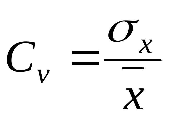
Коэффициент
вариации,
или изменчивости, годового
стока служит мерой оценки колебания
годовых величин стока относительно его
нормы и численно равен относительному
среднему
квадратическому отклонению
 .
.
Он служит также
для сравнения отдельных статистических
рядов, например годовых
величин стока разных рек, в отношении
их изменчивости
или рассеяния точек на кривой.
При
наличии длительных наблюдений Указаниями
СН 371-67 предусматриваются
два метода определения
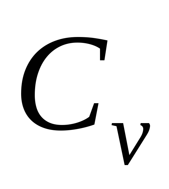
в зависимости от
изменчивости годового стока.
Если
изменчивость годового стока невелика
и характеризуется коэффициентом вариации
 ,
,
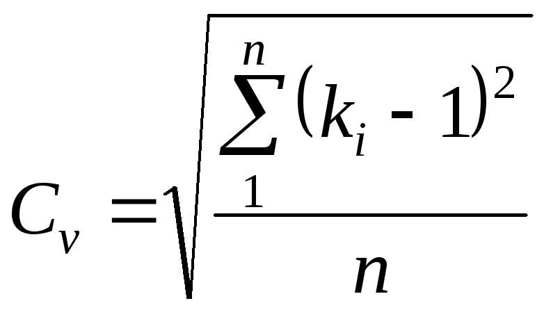
рекомендуется следующая
формула
 (3.1)
(3.1)
где
ki
– модульный
коэффициент стока каждого года; n
– число лет
наблюдений (число членов статистического
ряда).
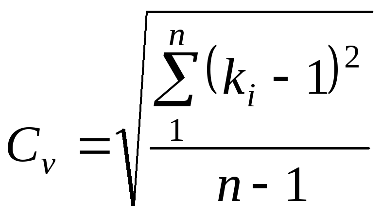
При
n<30
формула (3.1) используется в виде
 (3.1′)
Формула
(3.1) представляет собой выражение второго
момента
площади кривой распределения относительно
центральной ординаты,
а метод определения
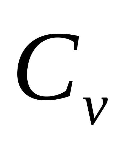 и
и

по
формулам (3.1 ) и
(3.6) называется методом моментов.
Относительная
средняя квадратическая ошибка коэффициента
вариации, вычисленная по этим формулам,
равна
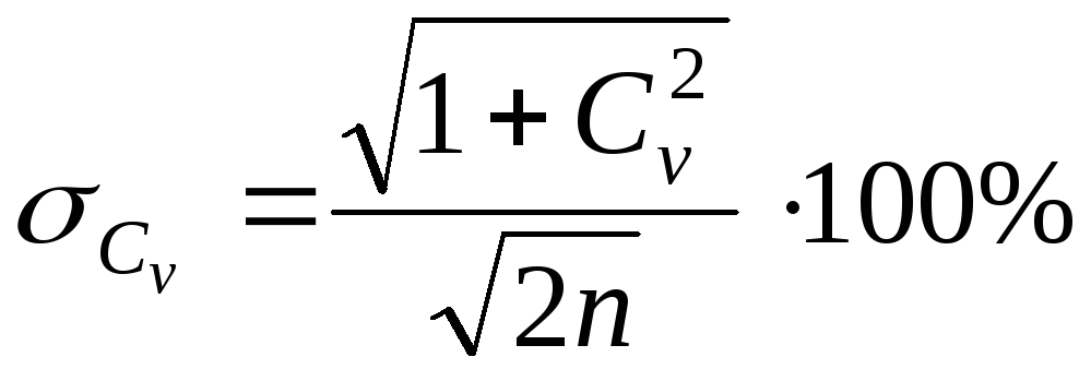 (3.2)
(3.2)
Формула
(4.2) предложена Е. Г. Блохиновым и
рекомендована Указаниями СН 371-67.
Для
нормального распределения параметра
или близкого к нему более обоснованной
формулой определения

является:
 (3.3)
(3.3)
Значения
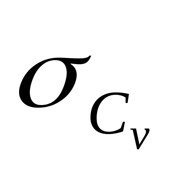
в зависимости
от п и
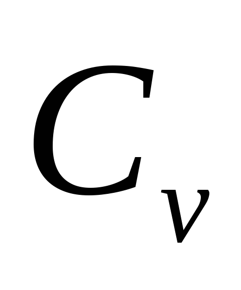
вычисленные по формулам (3.2) и (3.3),
приводятся в таблицах 3.1 и 3.2.
Таблица
3.1
Относительные
средние квадратические ошибки (%)
коэффициента вариации, вычисленные по
формуле (3.2)
|
|
Число |
|||||||||
|
10 |
20 |
30 |
40 |
50 |
60 |
70 |
80 |
90 |
100 |
|
|
0,20 |
23 |
16 |
13 |
11 |
10 |
9,3 |
8,6 |
8,1 |
7,6 |
7,2 |
|
0,30 |
23 |
17 |
14 |
12 |
10 |
9,6 |
8,8 |
8,3 |
7,8 |
7,4 |
|
0,40 |
24 |
17 |
14 |
12 |
11 |
9,8 |
9,1 |
8,5 |
8,0 |
7,6 |
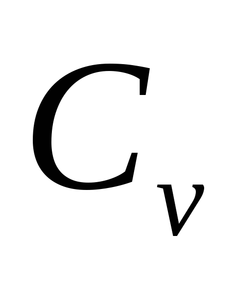
Примечание.
При
промежуточных значениях Cv
и
п
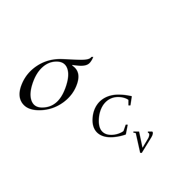 определяется
по
интерполяции.
Таблица
3.2
Относительные
средние квадратические ошибки (%)
коэффициента вариации, вычисленные по
формуле (3.3)
|
n |
|
||||
|
0,20 |
0,40 |
0,60 |
0,80 |
1,00 |
|
|
10 |
23,2 |
25 7 |
29,4 |
33,7 |
38,6 |
|
20 |
16,5 |
18,2 |
20,7 |
23,9 |
27,4 |
|
30 |
13,4 |
14,8 |
16,9 |
19,5 |
22,3 |
|
50 |
10,4 |
11,5 |
13,1 |
15,1 |
17,3 |
|
100 |
7,4 |
8,2 |
9,3 |
10,7 |
12,3 |

Из
этих таблиц видно, что для определения
 <0,50
<0,50
с точ-ностью ±10% необходимо иметь ряд
наблюдений продолжительностью 50—60
лет, а вычисления по формулам (3.2) и (3.3)
дают малую разницу, которая практически
не сказывается на конечных результатах
расчетов.
При
большой изменчивости годового стока
(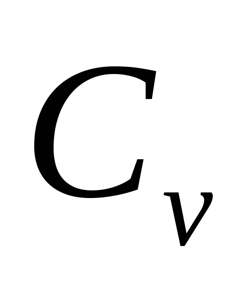 >0,50),
что характерно для рек засушливых
районов, коэффициент вариации определяется
методом наибольшего правдоподобия. По
этому методу значение Cv
устанавливается
в зависимости от параметра ,
который представляет собой среднее
значение логарифмов модульных
коэффициентов lg
k
и вычисляется по равенству
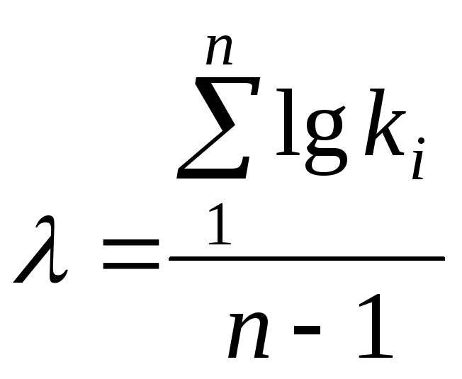 (3.4)
(3.4)
Имея
значение ,
по таблице 3.3 легко установить величину
Cv.
Относительная
средняя квадратическая ошибка Cv,
установленного
с помощью параметра ,
приближенно
равна
 (3.5)
(3.5)
Более
точные значения
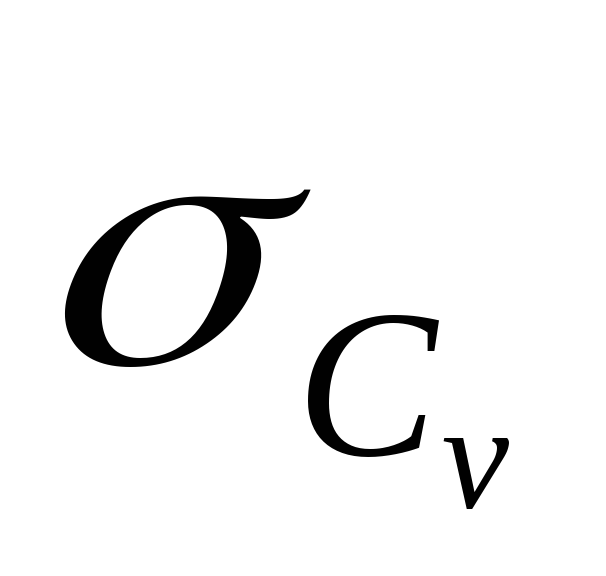 ,
,
вычисленные
методом наибольшего
правдоподобия, приводятся в таблице
3.4.
Значения
коэффициентов вариации, определенные
методом моментов
и методом наибольшего правдоподобия
при Сv
>0,5,
различаются
не более чем на 2–3% (таблица 3.4). В то же
время метод
наибольшего правдоподобия отличается
сложностью и громоздкостью
вычислений. Поэтому можно считать, что
метод наибольшего
правдоподобия для определения Cv
не
имеет преимущества перед методом
моментов и при массовых расчетах Cv
лучше пользоваться последним, т.е.
формулой (3.1),
который
оправдал себя при многочисленном
практическом применении.
Коэффициенты
вариации, установленные по формуле
(4.1)
и по
табл. 3.4 с помощью параметра ,
принимаются
в качестве расчетных,
когда их средняя квадратическая ошибка,
вычисленная
по формуле (3.2), не превышает следующие
пределы:
Интервалы
значений Cv
0,2—0,3
0,4—0,8 больше 0,8
Допустимая средняя
квадратическая
ошибка, %
20 10 5
Таблица
3.3
Относительная
средняя квадратическая ошибка (%)
коэффициента изменчивости
|
Cv |
Число |
|||||||||
|
10 |
20 |
30 |
40 |
50 |
60 |
70 |
80 |
90 |
100 |
|
|
0 50 |
21,5 |
15,2 |
12,4 |
10,8 |
9,6 |
8,8 |
8,1 |
7,6 |
7,2 |
6,8 |
|
0,75 |
20,5 |
14,5 |
11,8 |
10,3 |
9,2 |
8,4 |
7,7 |
7,2 |
6,9 |
6,5 |
|
1,00 |
19,4 |
13,7 |
11,2 |
9,7 |
8,7 |
7,9 |
7,3 |
6,8 |
6,5. |
6,1 |
|
1,25 |
18,2 |
12,8 |
10,5 |
9,1 |
8,1 |
7,5 |
6,9 |
6,4 |
6,1 |
5,8 |
|
1,50 |
16,9 |
12,0 |
9,8 |
8,5 |
7,6 |
6,9 |
6,4 |
6,0 |
5,7 |
5,4 |
|
1,75 |
15,8 |
11,2 |
9,1 |
7,9 |
7,0 |
6,4 |
6,0 |
5,6 |
5,3 |
5,0 |
|
2,00 |
14,6 |
10,4 |
8,4 |
7,3 |
6,6 |
6,0 |
5,5 |
5,2 |
4,9 |
4,6 |
Примечание.
При промежуточных значениях
Cv
и п средняя
квадра. тическая
ошибка определяется по интерполяции.
Таблица
3.4
Средние
значения Cv,
определенные
методами моментов и наибольшего
правдоподобия
-
Истинное
значение CvОбъем
выборки
иЗначение
Cvпо методу
моментовпо
методу наибольшего
правдоподобия0,25
0,50
1,00
25
50
25
50
25
50
0,25
0,24
0,49
0,50
0,97
0,98
0,25
0,25
0,49
0,50
0,99
1,00
Максимальные
ошибки Cv
значительно
превышают среднее квадратическос
значение. Они возможны тогда, когда в
короткий
ряд наблюдений, по которому определяются
Cv
, входит очень многоводный
или маловодный год, повторяемость
которого значительно
реже чем один раз в п
лет.
Однако вероятность больших
ошибок Cv,
в два-три раза превышающих ее среднюю
квадратическую
величину, очень мала.
Коэффициент
асимметрии
Cs
характеризует
несимметричность ряда
величин стока относительно его среднего
значения.
Это менее устойчивый параметр кривой
распределения
или обеспеченности и для надежного его
определения требуется
ряд наблюдений над стоком более 100—150
лет. По
имеющимся рядам наблюдений можно
установить лишь приближенное
значение коэффициента асимметрии. Для
этой цели используется формула третьего
момента
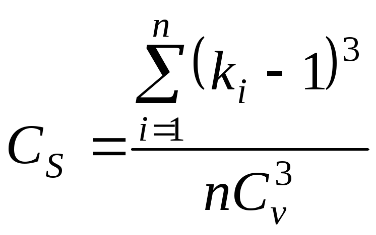 (3.6)
(3.6)
Относительная
средняя квадратическая ошибка Cs
зависит от
коэффициента вариации Сv
и числа лет наблюдений п.
Ее значение
при Cs
= 2Cv
с учетом
асимметричного распределения годовых
величин стока может быть определена по
формуле С. Н. Крицкого и М. Ф. Менкеля.
Так
при обычных значениях CV=0,20—0,40
средняя квадратичная ошибка
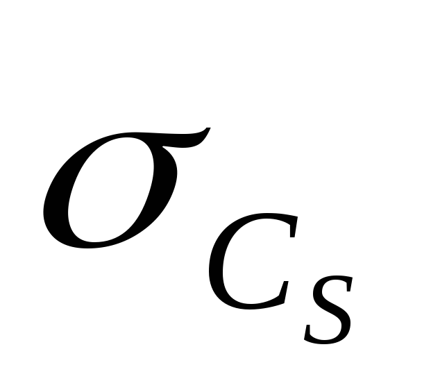
при
n=20—30
составляет около 14—16% от значения
коэффициента, а при n
= 50 уменьшается до 10—12%. Относительная
среднеквадратичная ошибка определения
коэффициента Cs
вычисляется
по формуле
 (3.7)
(3.7)
Величины
этих ошибок коэффициентов Cv
и
Cs,
определенных
по формулам (3.2-3.3) и (3.7), даны в таблицах
3.2–3.3 и 3.6.
Для
наиболее распространенных величин
годового стока рек лесной и лесостепной
зон Cv=0,20÷0,50.
Средняя ошибка его определения при
n=20-30
лет находится в пределах 15,5-19,5%.
Для
надежного подсчета коэффициента Сs
необходимо иметь, длительный ряд
(порядка
100
и
более), что практически бывает крайне
редко. Коэффициент обладaeт
более значительной устойчивостью во
времени и для надежного его подсчета
достаточен более короткий ряд наблюдении.
Поэтому обычно величину Сs
принимают
кратно значению Сv
т.е.
Сs=а
Сv (3.8)
Таблица
3.5
Относительные
средние квадратические ошибки определения
коэффициента асимметрии
 в % приСs
=2Cv
|
п |
Коэффициент |
|||||
|
0,10 |
0,20 |
0,40 |
126 |
0,80 |
1,00 |
|
|
10 |
399 |
216 |
140 |
126 |
126 |
134 |
|
20 |
281 |
153 |
99 |
85 |
89 |
95 |
|
30 |
234 |
125 |
80 |
72 |
74 |
78 |
|
40 |
199 |
108 |
70 |
63 |
64 |
67 |
|
50 |
178 |
96 |
63 |
56 |
57 |
60 |
|
100 |
125 |
69 |
44 |
39 |
41 |
42 |
Величина
а для
различных гидрологических характеристик
принимается различной. Так, для
биноминальной асимметричной кривой
пределом этой величины могут быть от
а=2 до
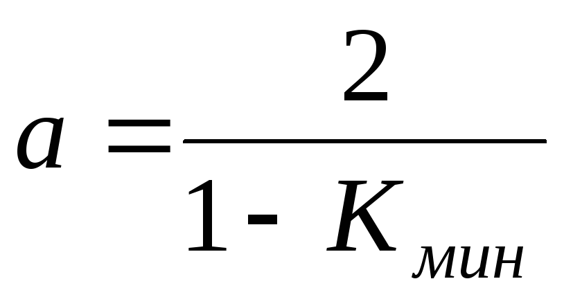 ;Кмин
;Кмин
– отношение
наинизшего расхода к среднему данного
ряда). Для среднегодового стока равенство
коэффициентов CS=Cv
справедливо
только при малых величинах Cv.
При больших
величинах
Cv
следует
применять
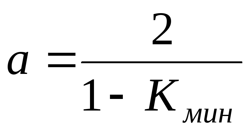 ,
,
что дает, как правило, величинуCS>2CV.
Для других
гидрологических величин соотношение
между Cv
и CS,
будет указано ниже.
При
наличии ряда наблюдений порядка 20 и
более построение кривой обеспеченности
выполняется с помощью таблицы
вспомогательных величин, образец которой
приведен в таблице. 3.6.
В
графе 12 подсчитывается обеспеченность
точек (модульных коэффициентов)
эмпирической кривой р
% определяется
по формуле
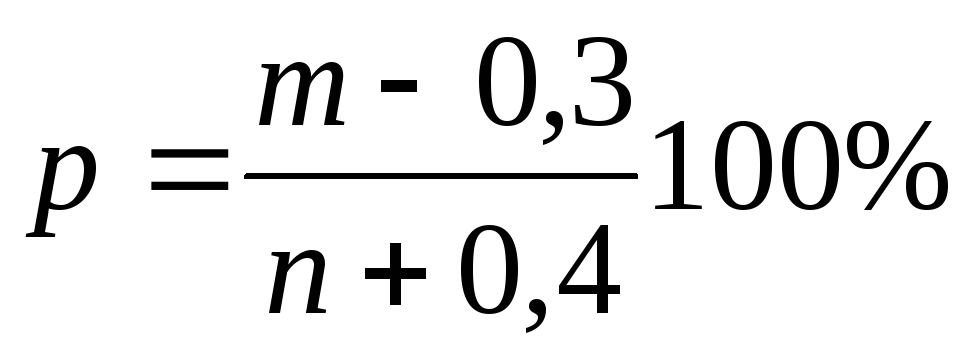 (3.9)
(3.9)
где
m
– порядковый номер члена ряда при
расположении их в убывающем порядке; n
– число членов в ряду.
Таблица
3.6
Вспомогательные
величины для построения кривой
обеспеченности
|
№ пп |
Год |
Q м3/сек |
в убывающ ем |
|
(k |
(k |
(k |
р, % |
|||
|
+ |
|
+ |
|
||||||||
|
годы |
Q, |
||||||||||
|
1 |
2 |
3 |
4 |
5 |
6 |
7 |
8 |
9 |
10 |
11 |
12 |
|
1 |
1894 |
1938 |
|||||||||
|
2 |
1895 |
1941 |
|||||||||
|
… |
… |
||||||||||
|
… |
1941 |
||||||||||
|
Сумма |
|
|
|
|
|
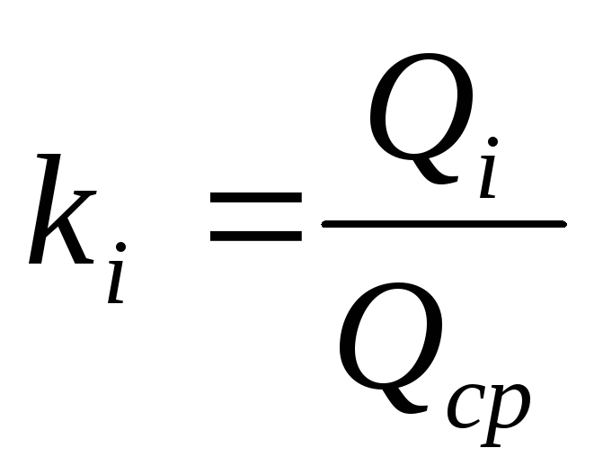

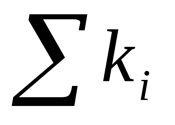

На
график (рис. 3.1) наносят точки ряда
наблюдений (полые кружки) и получают
кривую обеспеченности. Пользуясь табл.
3.6.можно построить на этом же графике
теоретическую кривую обеспеченности.
Для этого из графы 5 надо получить
величину  откуда
можно получить
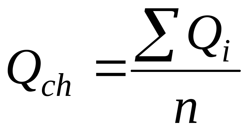
Для
контроля правильности подсчета сумма
модульных коэффициентов должна
удовлетворять равенству
 ,
,
а
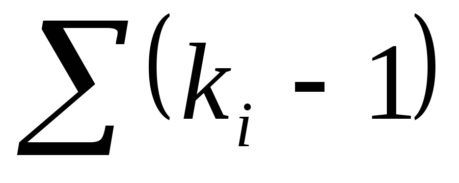
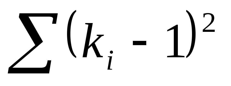
в графах 7, 8 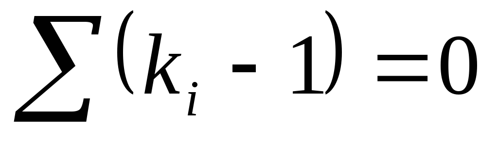 .Используя
сумму 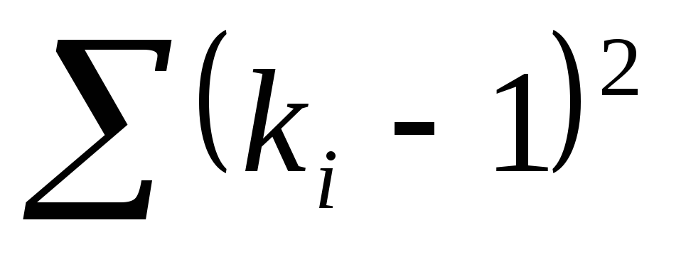 ,
,
из графы 9 можно получить значение
значение Cv
по
формуле (3.1-3.1′). В первом приближении
применяем CS=2CV.
Для
получения теоретических точек кривой
обеспеченности следует пользоваться
таблицей Фостера – Рыбкина, в которой
приведены отклонения ординат кривой
обеспеченности от середины Ф
при Хср
= 1 и Cv=1
(см. табл. 3.9).
Пользуясь
табл. 3.7, можно подсчитать значения
модульных коэффициентов по формуле
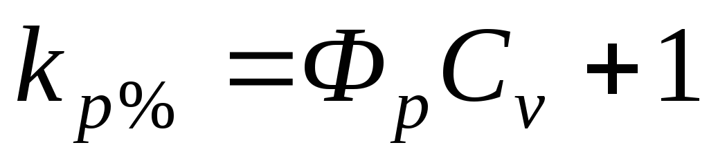 (3.10)
Затем
по формуле (4.5) определить значения
расходов разной обеспеченности:
 (3.11)
|
р, |
0,1 |
1 |
5 |
10 |
25 |
50 |
75 |
80 |
90 |
95 |
97 |
99 |
99,9 |
|
Сs=0,57 |
|||||||||||||
|
Фр |
|||||||||||||
|
Фр |
|||||||||||||
|
kp |
|||||||||||||
|
Qp |
|||||||||||||
|
kp |
|||||||||||||
|
Qp |
Результаты заносятся
в табл. 3.7.
Таблица 3.7
Полученные
значения Qр
– наносят
на график, приведенный на рис. 3.1 (на
рисунке значения Qр.
обозначены сплошными кружками). Если
проведенная по этим кружкам кривая
обеспеченности (пунктирная) не совпадает
с кривой, построенной по наблюденным
данным, то это обозначает, что принятое
значение Cs
для построения
теоретической кривой не соответствует
значению Cs
соответствующего
фактическим данным. Это значение
необходимо изменять до
тех
пор, пока теоретическая кривая не
совпадет с кривой натурных наблюдений.
Биноминальная
кривая обеспеченности хорошо согласуется
с натурными данными. Однако она имеет
ряд недостатков, одним из которых
является то, что при соотношении Cs
< 2 Cv
встречающемся на практике при расчетах
годового стока рек засушливых районов,
ординаты кривой обеспеченности в нижней
части имеют отрицательные значения.
Для исключения этого недостатка С. Н.
Крицкий и М. Ф. Менкель предложили новые
кривые обеспеченности [35]. По этим кривым
при любом соотношении Cs
и Cv
нулевая
ордината получается только при
обеспеченности в 100%. При CS=2CV
кривая
обеспеченности совпадает с биномальной
ассиметричной кривой.
Ассиметричные
кривые на
клетчатке вероятности спрямляются не
полностью и имеют выпуклость тем большую
, чем больше коэффициент асимметрии.
При положительной асимметрии выпуклость
обращена вниз, при отрицательной –
вверх.
Характеристика
связи между обеспеченностью и
повторяемостью расходов приведена в
табл. 3.8.
Применение
методов теории вероятности и математической
статистики
в решении гидрологических задач получило
широкое распространение как у нас, так
и за границей. Однако следует отметить
несовершенство
и условность этих методов. Кривые
обеспеченности, построенные теоретическим
путем, необходимо каждый раз анализировать
и проверять, используя фактические
наблюдения.

Рис.
3.1. Кривая обеспеченности средних годовых
расходов на клетчатке вероятности
Дальнейшее
развитие гидрологии должно идти по пути
все большего
развития генетических методов. Под ними
следует подразумевать
исследование закономерностей развития
гидрологических явлений и процессов
на основе обобщения данных наблюдений
и их физического анализа.
Таблица
3.8
Характеристики
лет
разной
обеспеченности
-
Обеспеченность,
%Повторяется
1
раз в n
летХарактеристика
года0,1
1000
Катастрофически
многоводный1
100
Очень многоводный
5
20
Многоводный
10
10
Средней
многоводности25
4
Средней
многоводности50
2
Медианный
75
4
Средней
маловодности90
10
Средней
маловодности95
20
Маловодный
97
33
Маловодный
99
100
Очень маловодный
99,9
1000
Катастрофически
маловодный
Таблица 3.9
Отклонение
ординат биноминальной асимметрической
кривой обеспеченности от середины (от
1,0) при Cv=1
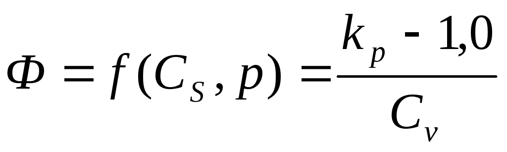
|
CS |
Обеспеченность |
CS |
|||||||||||||||||||
|
0,01 |
0,1 |
1 |
3 |
5 |
10 |
20 |
25 |
30 |
40 |
50 |
60 |
70 |
75 |
80 |
90 |
95 |
97 |
99 |
99,9 |
||
|
0,00 |
3,72 |
3,09 |
2,33 |
1,88 |
1,64 |
1,28 |
0,84 |
0,67 |
0,52 |
0,25 |
0,00 |
-0,25 |
-0,52 |
-0,67 |
-0,84 |
-1,28 |
-1,64 |
-1,88 |
-2,33 |
-3,09 |
0,00 |
|
0,05 |
3,83 |
3,16 |
2,36 |
1,90 |
1,65 |
1,28 |
0,84 |
0,66 |
0,52 |
0,24 |
-0,01 |
-0,26 |
-0,52 |
-0,68 |
-0,84 |
-1,28 |
-1,62 |
-1,86 |
-2,29 |
-3,02 |
0,05 |
|
0,10 |
3,94 |
3,23 |
2,40 |
1,92 |
1,67 |
1,29 |
0,84 |
0,66 |
0,51 |
0,24 |
-0,02 |
-0,27 |
-0,53 |
-0,68 |
-0,85 |
-1,27 |
-1,61 |
-1,81 |
-2,25 |
-2,95 |
0,10 |
|
0,15 |
4,05 |
3,31 |
2,44 |
194 |
1,68 |
1,30 |
0,84 |
0,66 |
0,50 |
0,23 |
-0,02 |
-0,28 |
-0,54 |
-0,68 |
-0,85 |
-1,26 |
-1,60 |
-1,82 |
-2,22 |
-2,88 |
0,15 |
|
0,20 |
4,16 |
3,38 |
2,47 |
1,96 |
1,70 |
1,30 |
0,83 |
0,65 |
050 |
0,22 |
-0,03 |
-0,28 |
-0,55 |
-0,69 |
-0,85 |
-1,26 |
-1,58 |
-1,79 |
-2,18 |
-2,81 |
0,20 |
|
0,25 |
4,27 |
3,45 |
2,50 |
1,98 |
1,71 |
1,30 |
0,82 |
0,64 |
0,49 |
0,21 |
-0,04 |
-0,29 |
-0,56 |
-0,70 |
-0,85 |
-1,25 |
-1,56 |
-1,77 |
-2,14 |
-2,74 |
0,25 |
|
0,30 |
4,38 |
3,52 |
2,54 |
2,00 |
1,72 |
1,31 |
0,82 |
0,64 |
0,48 |
0,20 |
-0,05 |
-0,30 |
-0,56 |
-0,70 |
-0,85 |
-1,24 |
-1,55 |
-1,75 |
-2,10 |
-2,67 |
0,30 |
|
0,35 |
4,50 |
3,59 |
2,58 |
2,02 |
1,73 |
1,32 |
0,82 |
0,64 |
0,48 |
0,20 |
-0,06 |
-0,30 |
0,56 |
-0,70 |
-0,85 |
-1,24 |
-1,53 |
-1,72 |
-2,06 |
-2,60 |
0,35 |
|
0,40 |
4,61 |
3,66 |
2,61 |
2,04 |
1,75 |
1,32 |
0,82 |
0,63 |
0,47 |
0,19 |
-0,07 |
-0,31 |
-0,57 |
-0,71 |
-0,85 |
-1,23 |
-1,52 |
-1,70 |
-2,03 |
-2,54 |
0,40 |
|
0,45 |
4,72 |
3,74 |
2,64 |
2,06 |
1,76 |
1,32 |
0,82 |
0,62 |
0,46 |
0,18 |
-0,08 |
-0,32 |
-0,58 |
-0,71 |
-0,85 |
-1,22 |
-1,51 |
-1,68 |
-2,00 |
-2,47 |
0,45 |
|
0,50 |
4,83 |
3,81 |
2,68 |
2,08 |
1,77 |
1,32 |
0,81 |
0,62 |
0,46 |
0,17 |
-0,08 |
-0,33 |
-0,58 |
-0,71 |
-0,85 |
-1,22 |
-1,49 |
-1,66 |
-1,99 |
-2,40 |
0,50 |
|
0,55 |
4,94 |
3,88 |
2,72 |
2,10 |
1,78 |
1,32 |
0,80 |
0,62 |
0,45 |
0,16 |
-0,09 |
-0,34 |
-0,58 |
-0,72 |
-0,85 |
-1,21 |
-1,47 |
-1,64 |
-1,92 |
-2,32 |
0,55 |
|
0,60 |
5,05 |
3,96 |
2,75 |
2,12 |
1,80 |
1,33 |
0,80 |
0,61 |
0,44 |
0,16 |
-0,10 |
-0,34 |
-0,59 |
0,72 |
-0,85 |
-1,20 |
-1,45 |
-1,61 |
-1,88 |
-2,27 |
0,60 |
|
0,65 |
5,16 |
4,03 |
2,78 |
2,14 |
1,81 |
1,33 |
0,80 |
0,60 |
0,44 |
0,15 |
-0,11 |
-0,35 |
-0,60 |
-0,72 |
-0,85 |
-1,44 |
1,19- |
1,59 |
-1,84 |
-2,20 |
0,65 |
|
0,70 |
5,28 |
4,10 |
2,82 |
2,15 |
1,82 |
1,33 |
0,79 |
0,59 |
0,43 |
0,14 |
-0,12 |
-0,36 |
-0,60 |
-0,72 |
-0,85 |
-1,18 |
-1,42 |
-1,57 |
-1,81 |
-2,14 |
0,70 |
|
0,75 |
5,39 |
4,17 |
2,86 |
2,16 |
1,83 |
1,34 |
0,78 |
0,58 |
0,42 |
0,13 |
-0,12 |
-0,36 |
-0,60 |
-0,72 |
-0,86 |
-1,18 |
-1,40 |
-1,54 |
-1,78 |
-2,08 |
0,75 |
|
0,80 |
5,50 |
4,24 |
2,89 |
2,18 |
1,84 |
1,34 |
0,78 |
0,58 |
0,41 |
0,12 |
-0,13 |
-0,37 |
-0,60 |
-0,73 |
-0,86 |
-1,17 |
-1,38 |
-1,52 |
-1,74 |
-2,02 |
0,80 |
|
0,85 |
5,62 |
4,31 |
2,92 |
2,20 |
1,85 |
1,34 |
0,78 |
0,58 |
0,40 |
0,12 |
-0,14 |
-0,38 |
-0,60 |
-0,73 |
-0,86 |
-1,16 |
-1,35 |
-,49 |
-1,70 |
-1,96 |
0,85 |
|
0,90 |
5,73 |
4,38 |
2,96 |
2,22 |
1,86 |
1,34 |
0,77 |
0,57 |
0,40 |
0,11 |
-0,15 |
-0,38 |
-0,61 |
-0,73 |
-0,85 |
-1,15 |
-1,35 |
-1,47 |
-1,66 |
-1,90 |
0,90 |
|
0,95 |
5,84 |
4,46 |
2,99 |
2,24 |
1,87 |
1,34 |
0,76 |
0,56 |
0,39 |
0,10 |
-0,16 |
-0,38 |
-0,62 |
-0,73 |
-0,85 |
-1,14 |
-1,34 |
-1,44 |
-1,62 |
-1,84 |
0,95 |
|
1,00 |
5,96 |
4,53 |
3,02 |
2,25 |
1,88 |
1,34 |
0,76 |
0,55 |
0,38 |
0,09 |
-0,16 |
-0,39 |
-0,62 |
-0,73 |
-0,85 |
-1,13 |
-1,32 |
-1,42 |
-1,59 |
-1,79 |
1,00 |
|
1,05 |
6,07 |
4,60 |
3,06 |
2,26 |
1,88 |
1,84 |
0,75 |
0,54 |
0,37 |
0,08 |
-0,17 |
-0,40 |
-0,62 |
-0,74 |
-0,85 |
-1,12 |
-1,30 |
-1,40 |
-1,56 |
-1,74 |
1,05 |
|
1,10 |
6,18 |
4,67 |
3,09 |
2,28 |
1,89 |
1,34 |
0,74 |
0,54 |
0,36 |
0,07 |
-0,18 |
-0,41 |
-0,62 |
-0,74 |
-0,85 |
-1,10 |
-1,28 |
-1,38 |
-1,52 |
-1,68 |
1,10 |
|
1,15 |
6,30 |
4,74 |
3,12 |
2,30 |
1,90 |
1,34 |
0,74 |
0,53 |
0,36 |
0,06 |
-0,18 |
-0,42 |
-0,62 |
-0,74 |
-0,84 |
-1,09 |
-1,26 |
-1,36 |
-1,48 |
-1,63 |
1,15 |
|
1,20 |
6,41 |
4,81 |
3,15 |
2,31 |
1,91 |
1,34 |
0,73 |
0,52 |
0,35 |
0,05 |
-0,19 |
-0,42 |
-0,63 |
-0,74 |
-0,84 |
-1,08 |
-1,24 |
-1,33 |
-1,45 |
-1,58 |
1,20 |
|
1,25 |
6,52 |
4,88 |
3,18 |
2,32 |
1,92 |
1,34 |
0,72 |
0,52 |
0,34 |
0,04 |
-0,20 |
-0,42 |
-0,63 |
-0,74 |
-0,84 |
-1,07 |
-1,22 |
-1,30 |
-1,42 |
-1,53 |
1,25 |
|
1,30 |
6,64 |
4,95 |
3,21 |
2,34 |
1,92 |
1,34 |
0,72 |
0,51 |
0,33 |
0,04 |
-0,21 |
-0,43 |
-0,63 |
-0,74 |
-0,84 |
-1,06 |
-1,20 |
-1,28 |
-1,38 |
-1,48 |
1,30 |
|
1,35 |
6,76 |
5,02 |
3,24 |
2,36 |
1,93 |
1,34 |
0,72 |
0,50 |
0,32 |
0,03 |
-0,22 |
-0,44 |
-0,64 |
-0,74 |
-0,84 |
-1,05 |
-1,18 |
-1,26 |
-1,35 |
-1,44 |
1,35 |
|
1,40 |
6,87 |
5,09 |
3,27 |
2,37 |
1,94 |
1,34 |
0,71 |
0,49 |
0,31 |
0,02 |
-0,22 |
-0,44 |
-0,64 |
-0,73 |
-0,83 |
-1,04 |
-1,17 |
-1,23 |
-1,32 |
-1,39 |
1,40 |
|
1,45 |
6,98 |
5,16 |
3,30 |
2,38 |
1,94 |
1,34 |
0,70 |
0,48 |
0,30 |
0,01 |
-0,23 |
-0,44 |
-0,64 |
-0,73 |
-0,82 |
-1,03 |
-1,15 |
-1,21 |
-1,29 |
-1,35 |
1,45 |
|
1,50 |
7,09 |
5,23 |
3,33 |
2,39 |
1,95 |
1,33 |
0,69 |
0,47 |
0,30 |
0,00 |
-0,24 |
-0,45 |
-0,64 |
-0,73 |
-0,82 |
-1,02 |
-1,13 |
-1,19 |
-1,26 |
-1,31 |
1,50 |
|
1,60 |
7,31 |
5,37 |
3,39 |
2,42 |
1,96 |
1,33 |
0,68 |
1,46 |
0,28 |
-0,02 |
-0,25 |
-0,46 |
-0,64 |
-0,73 |
-0,81 |
-0,99 |
-1,10 |
-1,14 |
-1,20 |
-1,24 |
1,60 |
Окончание
3.9
|
CS |
Обеспеченность |
CS |
|||||||||||||||||||
|
0,01 |
0,1 |
1 |
3 |
5 |
10 |
20 |
25 |
30 |
40 |
50 |
60 |
70 |
75 |
80 |
90 |
95 |
97 |
99 |
99,9 |
||
|
1,70 |
7,54 |
5,50 |
3,44 |
2,44 |
1,97 |
1,32 |
0,66 |
0,44 |
0,26 |
-0,03 |
-0,27 |
-0,47 |
-0,64 |
-0,72 |
-0,81 |
-0,97 |
-1,06 |
-1,10 |
-1,14 |
-1,17 |
1,70 |
|
1,80 |
7,76 |
5,64 |
3,50 |
2,46 |
1,98 |
1,32 |
0,64 |
0,42 |
0,24 |
-0,05 |
-0,28 |
-0,48 |
-0,64 |
-0,72 |
-0,80 |
-0,94 |
-1,02 |
-1,06 |
-1,09 |
-1,11 |
1,80 |
|
1,90 |
7,98 |
5,77 |
3,55 |
2,49 |
1,99 |
1,31 |
0,63 |
0,40 |
0,22 |
-0,07 |
-0,29 |
-0,48 |
-0,64 |
-0,72 |
-0,79 |
-0,92 |
-0,98 |
-1,01 |
-1,04 |
-1,05 |
1,90 |
|
2,0 |
8,21 |
5,91 |
3,60 |
2,51 |
2,00 |
1,30 |
0,61 |
0,39 |
0,20 |
-0,08 |
-0,31 |
-0,49 |
-0,64 |
-0,71 |
-0,78 |
-0,90 |
-,095 |
-0,97 |
-0,99 |
-1,00 |
2,0 |
|
2,10 |
— |
6,06 |
3,65 |
2,53 |
2,00 |
1,29 |
0,60 |
0,38 |
0,19 |
-0,01 |
-0,32 |
-0,49 |
-0,64 |
-0,70 |
-0,77 |
-0,87 |
-0,92 |
-0,94 |
-0,95 |
-0,95 |
2,10 |
|
2,20 |
— |
6,20 |
3,70 |
2,55 |
2,01 |
1,28 |
0,58 |
0,37 |
017 |
-0,11 |
-0,33 |
-0,49 |
-0,63 |
-0,69 |
-0,75 |
-0,85 |
-0,89 |
-0,90 |
-0,90 |
-0,91 |
2,20 |
|
2,30 |
— |
6,34 |
3,75 |
2,56 |
2,01 |
1,27 |
0,56 |
0,35 |
0,15 |
-0,12 |
-0,34 |
-0,49 |
-0,62 |
-0,68 |
-0,73 |
-0,82 |
-0,85 |
-0,86 |
-0,87 |
-0,87 |
2,30 |
|
2,40 |
— |
6,47 |
3,79 |
2,57 |
2,01 |
1,25 |
0,54 |
0,33 |
0,13 |
-0,14 |
-0,35 |
-0,50 |
-0,62 |
-0,66 |
-0,72 |
-0,79 |
-0,82 |
-0,83 |
-0,83 |
-0,83 |
2,40 |
|
2,50 |
— |
6,60 |
3,83 |
2,58 |
2,01 |
1,24 |
0,53 |
0,32 |
0,12 |
-0,15 |
-0,36 |
-0,50 |
-0,61 |
-0,65 |
-0,70 |
-0,77 |
-0,79 |
-0,80 |
-0,80 |
-0,80 |
2,50 |
|
2,60 |
— |
6,73 |
3,87 |
2,59 |
2,01 |
1,23 |
0,51 |
0,30 |
0,10 |
-0,17 |
-0,37 |
-0,50 |
-0,60 |
-0,64 |
-0,68 |
-0,74 |
-0,76 |
-0,76 |
-0,77 |
-0,77 |
2,60 |
|
2,70 |
— |
6,86 |
3,91 |
2,60 |
2,01 |
1,21 |
0,49 |
0,28 |
0,08 |
-0,18 |
-0,38 |
-0,50 |
-0,60 |
-0,63 |
-0,67 |
-0,72 |
-0,73 |
-0,74 |
-0,74 |
-0,74 |
2,70 |
|
2,80 |
— |
6,99 |
3,95 |
2,61 |
2,02 |
1,20 |
0,47 |
0,27 |
0,06 |
-0,20 |
-0,38 |
-0,50 |
-0,59 |
-0,62 |
-0,65 |
-0,70 |
-0,71 |
-0,71 |
-0,71 |
-0,71 |
2,80 |
|
2,90 |
— |
7,12 |
3,99 |
2,62 |
2,02 |
1,19 |
0,45 |
0,26 |
0,04 |
-0,21 |
-0,39 |
-0,50 |
-0,58 |
-0,61 |
-0,64 |
-0,67 |
-0,68 |
-0,69 |
-0,69 |
-0,69 |
2,90 |
|
3,00 |
— |
7,25 |
4,02 |
2,63 |
2,02 |
1,18 |
0,42 |
0,25 |
0,03 |
-0,23 |
-0,40 |
-0,50 |
-0,57 |
-0,61 |
-0,62 |
-0,65 |
-0,66 |
-0,66 |
-0,67 |
-0,67 |
3,00 |
|
3,10 |
— |
7,23 |
4,09 |
2,66 |
1,97 |
1,11 |
0,37 |
0,17 |
0,010 |
-0,23 |
-0,40 |
-0,51 |
-0,58 |
-0,60 |
-0,62 |
-0641 |
-0,645 |
-0,646 |
-0,646 |
-0,646 |
3,10 |
|
3,20 |
— |
7,35 |
4,11 |
2,66 |
1,96 |
1,09 |
0,35 |
0,15 |
-0,0006 |
-0,25 |
-0,41 |
-0,51 |
-0,57 |
-0,59 |
-0,61 |
-0,621 |
-0,625 |
-0,625 |
-0,625 |
-0,625 |
3,20 |
|
3,30 |
— |
7,44 |
4,15 |
2,66 |
1,95 |
1,08 |
0,33 |
0,13 |
-0,022 |
-0,26 |
-0,41 |
-0,50 |
-0,56 |
-0,58 |
-0,59 |
-0,605 |
-0,606 |
-0,606 |
-0,606 |
-0,606 |
3,30 |
|
3,40 |
— |
7,54 |
4,18 |
2,66 |
1,94 |
1,06 |
0,31 |
0,11 |
-0,036 |
-0,27 |
-0,41 |
-0,50 |
-0,55 |
-0,57 |
-0,58 |
-0,586 |
-0,587 |
-0,589 |
-0,589 |
-0,589 |
3,40 |
|
3,50 |
— |
7,64 |
4,21 |
2,66 |
1,93 |
1,04 |
0,29 |
0,085 |
-0,049 |
-0,28 |
-0,41 |
-0,50 |
-0,54 |
-0,55 |
-0,56 |
-0,57 |
-0,571 |
-0,571 |
-0,571 |
-0,571 |
3,50 |
|
3,60 |
— |
7,72 |
4,24 |
2,65 |
1,93 |
1,03 |
0,28 |
0,064 |
-0,072 |
-0,28 |
-0,42 |
-0,49 |
-0,54 |
-0,54 |
-0,55 |
-0,555 |
-0,556 |
-0,566 |
-0,556 |
0,552 |
3,60 |
|
3,70 |
— |
7,86 |
4,26 |
2,66 |
1,91 |
1,01 |
0,26 |
0,048 |
-0,084 |
-0,29 |
-0,42 |
-0,48 |
-0,52 |
-0,53 |
-0,54 |
-0,541 |
-0,541 |
-0,541 |
-0541 |
-0,541 |
3,70 |
|
3,80 |
— |
7,97 |
4,29 |
2,65 |
1,90 |
1,00 |
0,24 |
0,032 |
-0,095 |
-0,30 |
-0,42 |
-0,48 |
-0,51 |
-0,52 |
-0,52 |
-0,526 |
-0,526 |
-0,526 |
-0,526 |
-0,526 |
3,80 |
|
3,90 |
— |
8,08 |
4,32 |
2,65 |
1,90 |
0,98 |
0,23 |
0,020 |
-0,11 |
-0,30 |
-0,41 |
-0,47 |
-0,50 |
-0,51 |
-0,51 |
-0,513 |
-0,513 |
-0,513 |
-0,513 |
-0,513 |
3,90 |
|
4,00 |
— |
8,17 |
4,34 |
2,65 |
1,90 |
0,96 |
0,21 |
0,010 |
-0,12 |
-0,31 |
-0,41 |
-0,46 |
-0,49 |
-0,49 |
-0,50 |
-0,50 |
-0,50 |
-0,50 |
-0,50 |
-0,50 |
4,00 |
|
4,10 |
— |
8,29 |
4,36 |
2,65 |
1,89 |
0,95 |
0,20 |
0,000 |
-0,13 |
-0,31 |
-0,41 |
-0,46 |
-0,48 |
-0,484 |
-0,486 |
-0,487 |
-0,487 |
-0,487 |
-0,487 |
-0,487 |
4,10 |
|
4,20 |
— |
8,38 |
4,39 |
2,64 |
1,88 |
0,93 |
0,19 |
0,010 |
-0,13 |
-0,31 |
-0,41 |
-0,45 |
-0,47 |
-0,473 |
-0,476 |
-0,476 |
-0,476 |
-0,476 |
-0,476 |
-0,476 |
4,20 |
|
4,30 |
— |
8,49 |
4,40 |
2,64 |
1,87 |
0,92 |
0,17 |
0,021 |
-0,14 |
-0,32 |
-0,40 |
-0,44 |
-0,46 |
-0,462 |
-0,465 |
-0,465 |
-0,465 |
-0,465 |
-0,465 |
-0,465 |
4,30 |
|
4,40 |
— |
8,60 |
4,42 |
2,63 |
1,86 |
0,91 |
0,15 |
0,032 |
-0,15 |
-0,32 |
-0,40 |
-0,44 |
-0,451 |
-0,454 |
-0,455 |
-0,455 |
-0,455 |
-0,455 |
-0,455 |
-0,455 |
4,40 |
|
4,50 |
— |
8,69 |
4,44 |
2,62 |
1,85 |
0,89 |
0,14 |
0,042 |
-0,16 |
-0,32 |
-0,40 |
-0,43 |
-0,441 |
-0,444 |
-0,445 |
-0,445 |
-0,445 |
-0,445 |
-0,445 |
-0,445 |
4,50 |
|
4,60 |
— |
8,79 |
4,46 |
2,62 |
1,84 |
0,87 |
0,13 |
0,052 |
-0,17 |
-0,32 |
-0,40 |
-0,42 |
-0,432 |
-0,434 |
-0,435 |
-0,435 |
-0,435 |
-0,435 |
-0,435 |
-0,435 |
4,60 |
|
4,70 |
— |
8,89 |
4,49 |
2,61 |
1,83 |
0,85 |
0,11 |
0,064 |
-0,18 |
-0,32 |
-0,40 |
-0,42 |
-0,424 |
-0,425 |
-0,426 |
-0,426 |
-0,426 |
-0,426 |
-0,426 |
-0,426 |
4,70 |
|
4,80 |
— |
8,96 |
4,50 |
2,60 |
1,81 |
0,82 |
0,10 |
0,075 |
-0,19 |
-0,32 |
-0,39 |
-0,41 |
-0,416 |
-0,416 |
-0,416 |
-0,416 |
-0,416 |
-0,416 |
-0,416 |
-0,416 |
4,80 |
|
4,90 |
— |
9,04 |
4,51 |
2,60 |
1,80 |
0,80 |
0,084 |
0,087 |
-0,19 |
-0,33 |
-0,386 |
-0,401 |
-0,407 |
-0,408 |
-0,409 |
-0,409 |
-0,409 |
-0,409 |
-0,409 |
-0,409 |
4,90 |
|
5,00 |
— |
9,12 |
4,54 |
2,60 |
1,78 |
0,78 |
0,068 |
0,099 |
-0,20 |
-0,33 |
-0,380 |
-0,395 |
-0,399 |
-0,400 |
-0,400 |
-0,400 |
-0,400 |
-0,400 |
-0,400 |
-0,400 |
5,00 |
|
5,10 |
— |
9,20 |
4,57 |
2,60 |
1,76 |
0,76 |
0,051 |
0,11 |
-0,21 |
-0,33 |
-0,376 |
-0,388 |
-0,391 |
-0,392 |
-0,392 |
-0,392 |
-0,392 |
-0,392 |
-0,392 |
-0,392 |
5,10 |
|
5,20 |
— |
9,27 |
4,59 |
2,60 |
1,74 |
0,73 |
0,035 |
0,12 |
-0,21 |
-0,33 |
-0,370 |
-0,382 |
-0,384 |
-0,385 |
-0,385 |
-0,385 |
-0,385 |
-0,385 |
-0,385 |
-0,385 |
5,20 |
Таблица 3.10
Ординаты
биноминальной асимметрической кривой
обеспеченности kp
при CS
=2Cv
|
Cv |
Обеспеченность |
Cv |
|||||||||||||||||||
|
0,01 |
0,1 |
1 |
3 |
5 |
10 |
20 |
25 |
30 |
40 |
50 |
60 |
70 |
75 |
80 |
90 |
95 |
97 |
99 |
99,9 |
||
|
0,05 |
1,197 |
1,162 |
1,120 |
1,096 |
1,084 |
1,064 |
1,042 |
1,033 |
1,026 |
1,012 |
0,999 |
0,986 |
0,974 |
0,966 |
0,958 |
0,936 |
0,920 |
0,908 |
0,888 |
0,852 |
0,05 |
|
0,06 |
1,241 |
1,197 |
1,145 |
1,116 |
1,101 |
1,077 |
1,050 |
1,039 |
1,031 |
1,014 |
0,999 |
0,983 |
0,968 |
0,959 |
0,949 |
0,924 |
0,904 |
0,890 |
0,867 |
0,825 |
0,06 |
|
0,07 |
1,285 |
1,232 |
1,171 |
1,135 |
1,118 |
1,090 |
1,058 |
1,046 |
1,036 |
1,016 |
0,998 |
0,980 |
0,962 |
0,952 |
0,941 |
0,911 |
0,889 |
0,873 |
0,846 |
0,779 |
0,07 |
|
0,08 |
1,328 |
1,268 |
1,196 |
1,155 |
1,136 |
1,104 |
1,067 |
1,052 |
1,040 |
1,018 |
0,998 |
0,978 |
0,956 |
0,945 |
0,932 |
0,899 |
0,873 |
0,856 |
0,824 |
0,772 |
0,08 |
|
0,09 |
1,372 |
1,303 |
1,221 |
1,176 |
1,153 |
1,117 |
1,074 |
1,058 |
1,045 |
1,020 |
0,997 |
0,975 |
0,951 |
0,938 |
0,924 |
0,886 |
0,858 |
0,838 |
0,803 |
0,746 |
0,09 |
|
0,10 |
1,416 |
1,338 |
1,247 |
1,196 |
1,170 |
1,130 |
1,083 |
1,065 |
1,050 |
1,022 |
0,997 |
0,972 |
0,945 |
0,931 |
0,915 |
0,874 |
0,842 |
0,821 |
0,782 |
0,719 |
0,10 |
|
0,11 |
1,467 |
1,377 |
1,274 |
1,217 |
1,188 |
1,143 |
1,091 |
1,071 |
1,054 |
1,024 |
0,996 |
0,969 |
0,939 |
0,924 |
0,906 |
0,862 |
0,827 |
0,805 |
0,763 |
0,696 |
0,11 |
|
0,12 |
1,517 |
1,417 |
1,302 |
1,238 |
1,206 |
1,157 |
1,090 |
1,077 |
1,059 |
1,025 |
0,995 |
0,965 |
0,933 |
0,916 |
0,898 |
0,850 |
0,813 |
0,789 |
0,744 |
0,674 |
0,12 |
|
0,13 |
1,568 |
1,456 |
1,330 |
1,260 |
1,224 |
1,170 |
1,107 |
1,083 |
1,063 |
1,027 |
0,994 |
0,962 |
0,927 |
0,909 |
0,890 |
0,838 |
0,798 |
0,783 |
0,726 |
0,651 |
0,13 |
|
0,14 |
1,618 |
1,496 |
1,357 |
1,281 |
1,242 |
1,184 |
1,115 |
1,089 |
1,068 |
1,028 |
0,993 |
0,958 |
0,921 |
0,902 |
0,881 |
0,826 |
0,784 |
0,757 |
0,707 |
0,628 |
0,14 |
|
0,15 |
1,669 |
1,535 |
1,384 |
1,302 |
1,260 |
1,197 |
1,124 |
1,096 |
1,072 |
1,030 |
0,992 |
0,955 |
0,916 |
0,894 |
0,872 |
0,814 |
0,769 |
0,740 |
0,688 |
0,606 |
0,15 |
|
0,16 |
1,720 |
1,574 |
1,412 |
1,323 |
1,278 |
1,210 |
1,132 |
1,101 |
1,076 |
1,032 |
0,990 |
0,952 |
0,910 |
0,887 |
0,864 |
0,802 |
0,754 |
0,724 |
0,669 |
0,583 |
0,16 |
|
0,17 |
1,770 |
1,614 |
1,440 |
1,344 |
1,296 |
1,224 |
1,140 |
1,108 |
1,081 |
1,033 |
0,989 |
0,948 |
0,904 |
0,880 |
0,856 |
0,790 |
0,740 |
0,708 |
0,650 |
0,560 |
0,17 |
|
0,18 |
1,821 |
1,653 |
1,467 |
1,366 |
1,314 |
1,237 |
1,148 |
1,114 |
1,085 |
1,035 |
0,988 |
0,945 |
0,898 |
0,873 |
0,847 |
0,778 |
0,725 |
0,692 |
0,632 |
0,537 |
0,18 |
|
0,19 |
1,871 |
1,693 |
1,494 |
1,387 |
1,332 |
1,251 |
1,156 |
1,120 |
1,090 |
1,036 |
0,987 |
0,941 |
0,892 |
0,865 |
0,838 |
0,766 |
0,711 |
0,676 |
0,613 |
0,515 |
0,19 |
|
0,20 |
1,922 |
1,732 |
1,522 |
1,408 |
1,350 |
1,264 |
1,164 |
1,126 |
1,094 |
1,038 |
0,986 |
0,938 |
0,886 |
0,858 |
0,830 |
0,754 |
0,696 |
0,660 |
0,594 |
0,492 |
0,20 |
|
0,21 |
1,981 |
1,778 |
1,552 |
1,431 |
1,369 |
1,278 |
1,172 |
1,132 |
1,098 |
1,039 |
0,984 |
0,934 |
0,880 |
0,851 |
0,822 |
0,743 |
0,683 |
0,646 |
0,578 |
0,475 |
0,21 |
|
0,22 |
2,041 |
1,823 |
1,582 |
1,454 |
1,388 |
1,291 |
1,179 |
1,137 |
1,102 |
1,040 |
0,983 |
0,930 |
0,873 |
0,843 |
0,813 |
0,731 |
0,670 |
0,631 |
0,562 |
1,457 |
0,22 |
|
0,23 |
2,100 |
1,869 |
1,613 |
1,476 |
1,407 |
1,304 |
1,187 |
1,142 |
1,105 |
1,041 |
0,981 |
0,926 |
0,867 |
0,836 |
0,804 |
0,720 |
0,657 |
0,617 |
0,547 |
0,440 |
0,23 |
|
0,24 |
2,159 |
1,914 |
1,643 |
1,499 |
1,426 |
1,318 |
1,194 |
1,149 |
1,109 |
1,042 |
0,980 |
0,922 |
0,861 |
0828 |
0,796 |
0,708 |
0,644 |
0,603 |
0,531 |
0,423 |
0,24 |
|
0,25 |
2,218 |
1,960 |
1,674 |
1,522 |
1,445 |
1,332 |
1,202 |
1,154 |
1,113 |
1,043 |
0,978 |
0,918 |
0,854 |
0,821 |
0,788 |
0,697 |
0,630 |
0,588 |
0,515 |
0,406 |
0,25 |
|
0,26 |
2,278 |
2,006 |
1,704 |
1,545 |
1,464 |
1,345 |
1,210 |
1,160 |
1,117 |
1,044 |
0,976 |
0,914 |
0,848 |
0,814 |
0,779 |
0,686 |
0,617 |
0,574 |
0,499 |
0,388 |
0,26 |
|
0,27 |
2,337 |
2,051 |
1,734 |
1,568 |
1,483 |
1,358 |
1,217 |
1,166 |
1,121 |
1,045 |
0,975 |
0,910 |
0,842 |
0,806 |
0,770 |
0,674 |
0,604 |
0,560 |
0,483 |
0,371 |
0,27 |
|
0,28 |
2,396 |
2,097 |
1,764 |
1,590 |
1,502 |
1,372 |
1,225 |
1,172 |
1,124 |
1,046 |
0,973 |
0,906 |
0,836 |
0,799 |
0,762 |
0,663 |
0,591 |
0,546 |
0,468 |
0,354 |
0,28 |
|
0,29 |
2,456 |
2,142 |
1,795 |
1,613 |
1,521 |
1,386 |
1,232 |
1,177 |
1,128 |
1,047 |
0,972 |
0,902 |
0,829 |
0,791 |
0,754 |
0,651 |
0,578 |
0,531 |
0,452 |
0,336 |
0,29 |
|
0,30 |
2,515 |
2,188 |
1,825 |
1,636 |
1,540 |
1,399 |
1,240 |
1,183 |
1,132 |
1,048 |
0,970 |
0,898 |
0,823 |
0,784 |
0,745 |
0,640 |
0,564 |
0,517 |
0,436 |
0,319 |
0,30 |
|
0,31 |
2,584 |
2,239 |
1,858 |
1,660 |
1,560 |
1,413 |
1,247 |
1,188 |
1,135 |
1,048 |
0,968 |
0,893 |
0,817 |
0,776 |
0,736 |
0,629 |
0,553 |
0,504 |
0,423 |
0,306 |
0,31 |
|
0,32 |
2,662 |
2,290 |
1,891 |
1,683 |
1,579 |
1,426 |
1,254 |
1,193 |
1,138 |
1,048 |
0,966 |
0,889 |
0,810 |
0,769 |
0,727 |
0,618 |
0,542 |
0,492 |
0,410 |
0,294 |
0,32 |
|
0,33 |
2,721 |
2,340 |
1,924 |
1,707 |
1,599 |
1,440 |
1,262 |
1,198 |
1,142 |
1,048 |
0,963 |
0,884 |
0,804 |
0,761 |
0,718 |
0,608 |
0,530 |
0,480 |
0,396 |
0,281 |
0,33 |
|
0,34 |
2,789 |
2,391 |
1,957 |
1,730 |
1,618 |
1,454 |
1,269 |
1,203 |
1,145 |
1,048 |
0,961 |
0,880 |
0,798 |
0,754 |
0,709 |
0,597 |
0,518 |
0,467 |
0,383 |
0,268 |
0,34 |
|
0,35 |
2,858 |
2,442 |
1,990 |
1,754 |
1,638 |
1,468 |
1,276 |
1,208 |
1,148 |
1,048 |
0,959 |
0,875 |
0,792 |
0,746 |
0,700 |
0,586 |
0,506 |
0,454 |
0,370 |
0,256 |
0,35 |
|
0,36 |
2,926 |
2,493 |
2,024 |
1,778 |
1,658 |
1,481 |
1,283 |
1,212 |
1,151 |
1,048 |
0,957 |
0,870 |
0,785 |
0,738 |
0,692 |
0,575 |
0,495 |
0,442 |
0,357 |
0,243 |
0,36 |
Продолжение
табл.3.10
|
Cv |
Обеспеченность |
Cv |
|||||||||||||||||||
|
0,01 |
0,1 |
1 |
3 |
5 |
10 |
20 |
25 |
30 |
40 |
50 |
60 |
70 |
75 |
80 |
90 |
95 |
97 |
99 |
99,9 |
||
|
0,37 |
2,994 |
2,544 |
2,057 |
1,801 |
1,677 |
1,495 |
1,290 |
1,217 |
1,154 |
1,048 |
0,955 |
0,866 |
0,779 |
0,731 |
0,683 |
0,564 |
0,483 |
0,430 |
0,344 |
0,230 |
0,37 |
|
0,38 |
30,063 |
2,594 |
2,090 |
1,825 |
1,697 |
1,509 |
1,298 |
1,222 |
1,158 |
1,048 |
0,952 |
0,861 |
0,773 |
0,723 |
0,674 |
0,554 |
0,471 |
0,417 |
0,330 |
0,217 |
0,38 |
|
0,39 |
3,132 |
2,645 |
2,123 |
1,848 |
1,716 |
1,522 |
1,305 |
1,227 |
1,161 |
1,048 |
0,950 |
0,857 |
0,769 |
0,716 |
0,665 |
0,543 |
0,460 |
0,404 |
0,317 |
0,205 |
0,39 |
|
0,40 |
3,200 |
2,696 |
2,156 |
1,872 |
1,736 |
1,536 |
1,312 |
1,232 |
1,164 |
1,048 |
0,948 |
0,852 |
0,766 |
0,708 |
0,656 |
0,533 |
0,448 |
0,392 |
0,304 |
0,192 |
0,40 |
|
0,41 |
3,278 |
2,753 |
2,192 |
1,897 |
1,756 |
1,549 |
1,319 |
1,236 |
1,167 |
1,048 |
0,945 |
0,847 |
0,753 |
0,701 |
0,648 |
0,522 |
0,437 |
0,382 |
0,294 |
0,184 |
0,41 |
|
0,42 |
3,356 |
2,810 |
2,227 |
1,923 |
1,776 |
1,563 |
1,325 |
1,241 |
1,169 |
1,047 |
0,942 |
0,842 |
0,746 |
0,693 |
0,640 |
0,513 |
0,427 |
0,371 |
0,284 |
0,175 |
0,42 |
|
0,43 |
3,433 |
2,867 |
2,262 |
1,948 |
1,797 |
1,576 |
1,332 |
1,246 |
1,172 |
1,047 |
0,939 |
0,837 |
0,739 |
0,686 |
0,631 |
0,503 |
0,416 |
0,361 |
0,275 |
0,166 |
0,43 |
|
0,44 |
3,511 |
2,924 |
2,298 |
1,974 |
1,817 |
1,590 |
1,338 |
1,250 |
1,174 |
1,046 |
0,936 |
0,832 |
0,732 |
0,678 |
0,623 |
0,494 |
0,406 |
0,350 |
0,265 |
0,158 |
0,44 |
|
0,45 |
3,589 |
2,981 |
2,334 |
1,999 |
1,837 |
1,603 |
1,345 |
1,254 |
1,177 |
1,046 |
0,933 |
0,828 |
0,726 |
0,671 |
0,615 |
0,484 |
0,395 |
0,340 |
0,255 |
0,150 |
0,45 |
|
0,46 |
3,667 |
3,038 |
2,369 |
2,024 |
1,857 |
1,616 |
1,352 |
1,259 |
1,180 |
1,046 |
0,930 |
0,823 |
0,719 |
0,664 |
0,607 |
0,474 |
0,384 |
0,330 |
0,245 |
0,141 |
0,46 |
|
0,47 |
3,745 |
3,095 |
2,404 |
2,050 |
1,877 |
1,630 |
1,358 |
1,264 |
1,182 |
1,045 |
0,927 |
0,818 |
0,712 |
0,656 |
0,599 |
0,465 |
0,374 |
0,319 |
0,236 |
0,132 |
0,47 |
|
0,48 |
3,822 |
3,152 |
2,440 |
2,075 |
1,898 |
1,643 |
1,365 |
1,268 |
1,185 |
1,045 |
0,924 |
0,813 |
0,705 |
0,649 |
0,590 |
0,455 |
0,363 |
0,309 |
0,226 |
0,126 |
0,48 |
|
0,49 |
3,900 |
3,209 |
2,476 |
2,101 |
1,918 |
1,657 |
1,371 |
1,272 |
1,187 |
1,044 |
0,921 |
0,808 |
0,698 |
0,641 |
0,582 |
0,446 |
0,353 |
0,298 |
0,216 |
0,116 |
0,49 |
|
0,50 |
3,978 |
3,226 |
2,511 |
2,126 |
1,938 |
1,670 |
1,378 |
1,277 |
1,190 |
1,044 |
0,918 |
0,803 |
0,691 |
0,634 |
0,574 |
0,436 |
0,342 |
0,288 |
0,206 |
0,107 |
0,50 |
|
0,51 |
4,065 |
3,328 |
2,549 |
2,152 |
1,959 |
1,683 |
1,384 |
1,280 |
1,192 |
1,043 |
0,915 |
0,798 |
0,684 |
0,626 |
0,566 |
0,428 |
0,333 |
0,279 |
0,198 |
0,102 |
0,51 |
|
0,52 |
4,152 |
3,390 |
2,587 |
2,178 |
1,980 |
1,697 |
1,390 |
1,284 |
1,191 |
1,041 |
0,912 |
0,792 |
0,677 |
0,618 |
0,558 |
0,419 |
0,325 |
0,271 |
0,191 |
0,096 |
0,52 |
|
0,53 |
4,238 |
3,452 |
2,625 |
2,204 |
2,000 |
1,710 |
1,396 |
1,288 |
1,196 |
1,040 |
0,908 |
0,786 |
0,670 |
0,611 |
0,551 |
0,411 |
0,316 |
0,262 |
0,0183 |
0,090 |
0,53 |
|
0,54 |
4,325 |
3,514 |
2,663 |
2,230 |
2,0021 |
1,724 |
1,402 |
1,291 |
1,198 |
1,038 |
0,905 |
0,781 |
0,663 |
0,603 |
0,543 |
0,402 |
0,308 |
0,254 |
0,176 |
0,085 |
0,54 |
|
0,55 |
4,412 |
3,576 |
2,700 |
2,256 |
2,042 |
1,737 |
1,408 |
1,294 |
1,200 |
1,037 |
0,902 |
0,776 |
0,656 |
0,595 |
0,535 |
0,394 |
0,299 |
0,245 |
0,168 |
0,080 |
0,55 |
|
0,56 |
4,499 |
3,638 |
2,738 |
2,282 |
2,063 |
1,750 |
1,414 |
1,298 |
1,202 |
1,036 |
0,899 |
0,770 |
0,650 |
0,587 |
0,527 |
0,386 |
0,290 |
0,236 |
0,160 |
0,074 |
0,56 |
|
0,57 |
4,586 |
3,700 |
2,776 |
2,308 |
2,084 |
1,764 |
1,420 |
1,302 |
1,204 |
1,034 |
0,896 |
0,765 |
0,643 |
0,579 |
0,519 |
0,377 |
0,282 |
0,228 |
0,153 |
0,068 |
0,57 |
|
0,58 |
4,672 |
3,762 |
2,814 |
2,334 |
2,104 |
1,777 |
1,426 |
1,305 |
1,206 |
1,033 |
0,892 |
0,759 |
0,636 |
0,572 |
0,512 |
0,369 |
0,273 |
0,219 |
0,145 |
0,063 |
0,58 |
|
0,59 |
4,759 |
3,824 |
2,852 |
2,360 |
2,125 |
1,791 |
1,432 |
1,308 |
1,208 |
1,031 |
0,889 |
0,754 |
0,629 |
0,564 |
0,504 |
0,360 |
0,265 |
0,211 |
0,0138 |
0,058 |
0,59 |
|
0,60 |
4,846 |
3,886 |
2,890 |
2,386 |
2,146 |
1,804 |
1,438 |
1,312 |
1,210 |
1,030 |
0,886 |
0,748 |
0,622 |
0,556 |
0,496 |
0,352 |
0,256 |
0,202 |
0,130 |
0,052 |
0,60 |
|
0,61 |
4,942 |
3,954 |
2,930 |
2,413 |
2,167 |
1,817 |
1,444 |
1,315 |
1,211 |
1,028 |
0,882 |
0,742 |
0,615 |
0,549 |
0,488 |
0,344 |
0,248 |
0,196 |
0,125 |
0,050 |
0,61 |
|
0,62 |
5,039 |
4,021 |
2,970 |
2,441 |
2,188 |
1,831 |
1,450 |
1,318 |
1,211 |
1,027 |
0,878 |
0,737 |
0,608 |
0,543 |
0,481 |
0,336 |
0,241 |
0,189 |
0,119 |
0,047 |
0,62 |
|
0,63 |
5,135 |
4,089 |
3,010 |
2,468 |
2,210 |
1,844 |
1,456 |
1,321 |
1,212 |
10,25 |
0,874 |
0,731 |
0,601 |
0,536 |
0,473 |
0,328 |
0,234 |
0,183 |
0,114 |
0,044 |
0,63 |
|
0,64 |
5,231 |
4,157 |
3,050 |
2,495 |
2,231 |
1,858 |
1,462 |
1,324 |
1,213 |
1,024 |
0,870 |
0,726 |
0,594 |
0,529 |
0,465 |
0,320 |
0,226 |
0,177 |
0,108 |
0,042 |
0,64 |
|
0,65 |
5,328 |
4,224 |
3,090 |
2,522 |
2,252 |
1,871 |
1,468 |
1,328 |
1,214 |
1,022 |
0,866 |
0,720 |
0,587 |
0,522 |
0,458 |
0,312 |
0,218 |
0,170 |
0,103 |
0,040 |
0,65 |
|
0,66 |
5,424 |
4,292 |
3,129 |
2,550 |
2,273 |
1,884 |
1,473 |
1,331 |
1,214 |
1,020 |
0,862 |
0,714 |
0,580 |
0,516 |
0,450 |
0,304 |
0,211 |
0,164 |
0,098 |
0,037 |
0,66 |
|
0,67 |
5,520 |
4,360 |
3,169 |
2,577 |
2,294 |
1,898 |
1,479 |
1,334 |
1,215 |
1,019 |
0,858 |
0,709 |
0,573 |
0,509 |
0,442 |
0,296 |
0,204 |
0,158 |
0,092 |
0,034 |
0,67 |
|
0,68 |
5,616 |
4,428 |
30,209 |
2,604 |
2,316 |
1,911 |
1,485 |
1,337 |
1,216 |
1,017 |
0,854 |
0,703 |
0,566 |
0,502 |
0,434 |
0,288 |
0,196 |
0,152 |
0,087 |
0,032 |
0,68 |
|
0,69 |
5,713 |
4,495 |
3,249 |
2,632 |
2,337 |
1,925 |
1,491 |
1,339 |
1,216 |
1,016 |
0,850 |
0,698 |
0,559 |
0,496 |
0,427 |
0,280 |
0,188 |
0,145 |
0,081 |
0,030 |
0,69 |
|
0,70 |
5,809 |
4,563 |
3,289 |
2,659 |
2,358 |
1,938 |
1,497 |
1,343 |
1,217 |
1,014 |
0,846 |
0,692 |
0,552 |
0,489 |
0,419 |
0,272 |
0,181 |
0,139 |
0,076 |
0,027 |
0,70 |
|
0,71 |
5,913 |
4,636 |
3,331 |
2,687 |
2,379 |
1,951 |
1,502 |
1,346 |
1,218 |
1,011 |
0,841 |
0,686 |
0,546 |
0,482 |
0,412 |
0,266 |
0,175 |
0,134 |
0,072 |
0,025 |
0,71 |
Продолжение
табл.3.10
|
Cv |
Обеспеченность |
Cv |
|||||||||||||||||||
|
0,01 |
0,1 |
1 |
3 |
5 |
10 |
20 |
25 |
30 |
40 |
50 |
60 |
70 |
75 |
80 |
90 |
95 |
97 |
99 |
99,9 |
||
|
0,72 |
6,017 |
4,710 |
3,374 |
2,714 |
2,400 |
1,963 |
1,506 |
1,348 |
1,218 |
1,008 |
0,837 |
0,680 |
0,539 |
0,474 |
0,406 |
0,259 |
0,168 |
0,129 |
0,069 |
0,023 |
0,72 |
|
0,73 |
6,121 |
4,783 |
3,416 |
2,742 |
2,421 |
1,976 |
1,511 |
1,350 |
1,219 |
1,005 |
0,832 |
0,674 |
0,533 |
0,467 |
0,399 |
0,253 |
0,163 |
0,124 |
0,065 |
0,021 |
0,73 |
|
0,74 |
6,225 |
4,856 |
3,458 |
2,770 |
2,442 |
1,988 |
1,516 |
1,353 |
1,220 |
1,002 |
0,828 |
0,668 |
0,526 |
0,460 |
0,392 |
0,246 |
0,157 |
0,119 |
0,062 |
0,019 |
0,74 |
|
0,75 |
6,328 |
4,930 |
3,500 |
2,798 |
2,463 |
2,001 |
1,520 |
1,356 |
1,220 |
0,999 |
0,823 |
0,662 |
0,520 |
0,452 |
0,386 |
0,240 |
0,150 |
0,113 |
0,058 |
0,018 |
0,75 |
|
0,76 |
6,432 |
5,003 |
3,543 |
2,825 |
2,484 |
2,014 |
1,525 |
1,358 |
1,221 |
0,996 |
0,818 |
0,656 |
0,514 |
0,445 |
0,379 |
0,234 |
0,144 |
0,108 |
0,054 |
0,016 |
0,76 |
|
0,77 |
6,536 |
5,076 |
3,585 |
2,853 |
2,505 |
2,026 |
1,530 |
1,360 |
1,222 |
0,993 |
0,814 |
0,650 |
0,507 |
0,438 |
0,372 |
0,227 |
0,138 |
0,103 |
0,051 |
0,014 |
0,77 |
|
0,78 |
6,640 |
5,149 |
3,627 |
2,881 |
2,526 |
2,039 |
1,535 |
1,363 |
1,223 |
0,990 |
0,809 |
0,644 |
0,501 |
0,431 |
0,365 |
0,221 |
0,132 |
0,098 |
0,047 |
0,012 |
0,78 |
|
0,79 |
6,744 |
5,223 |
3,670 |
2,908 |
2,547 |
2,051 |
1,539 |
1,366 |
1,223 |
0,987 |
0,805 |
0,638 |
0,494 |
0,423 |
0,359 |
0,214 |
0,126 |
0,093 |
0,044 |
0,010 |
0,79 |
|
0,80 |
6,848 |
5,296 |
3,712 |
2,936 |
2,568 |
2,064 |
1,544 |
1,368 |
1,224 |
0,984 |
0,800 |
0,632 |
0,488 |
0,416 |
0,352 |
0,208 |
0,120 |
0,088 |
0,040 |
0,008 |
0,80 |
|
0,81 |
6,962 |
5,374 |
3,756 |
2,964 |
2,589 |
2,076 |
1,547 |
1,369 |
1,223 |
0,981 |
0,795 |
0,626 |
0,482 |
0,410 |
0,345 |
0,203 |
0,116 |
0,084 |
0,038 |
0,007 |
0,81 |
|
0,82 |
7,075 |
5,452 |
3,800 |
2,992 |
2,611 |
2,089 |
1,550 |
1,370 |
1,222 |
0,978 |
0,790 |
0,619 |
0,475 |
0,403 |
0,338 |
0,197 |
0,112 |
0,080 |
0,036 |
0,007 |
0,82 |
|
0,83 |
0,189 |
5,530 |
3,843 |
3,019 |
2,632 |
2,101 |
1,554 |
1,371 |
1,222 |
0,975 |
0,784 |
0,613 |
0,469 |
0,397 |
0,330 |
0,192 |
0,109 |
0,075 |
0,034 |
0,006 |
0,83 |
|
0,84 |
7,302 |
5,608 |
3,887 |
2,047 |
2,654 |
2,114 |
1,557 |
1,372 |
1,221 |
0,972 |
0,779 |
0,606 |
0,462 |
0,390 |
0,323 |
0,186 |
0,105 |
0,071 |
0,032 |
0,006 |
0,84 |
|
0,85 |
7,416 |
5,686 |
3,931 |
3,075 |
2,675 |
2,126 |
1,546 |
1,373 |
1,220 |
0,970 |
0,774 |
0,600 |
0,456 |
0,384 |
0,316 |
0,181 |
0,0101 |
0,067 |
0,030 |
0,005 |
0,85 |
|
0,86 |
7,530 |
5,764 |
3,975 |
3,103 |
2,696 |
2,138 |
1,563 |
1,374 |
1,219 |
0,967 |
0,769 |
0,594 |
0,450 |
0,378 |
0,309 |
0,176 |
0,097 |
0,063 |
0,027 |
0,004 |
0,86 |
|
0,87 |
7,643 |
5,542 |
4,019 |
3,131 |
2,718 |
2,151 |
1,566 |
1,375 |
1,218 |
0,964 |
0,764 |
0,587 |
0,443 |
0,371 |
0,302 |
0,170 |
0,093 |
0,058 |
0,025 |
0,004 |
0,87 |
|
0,88 |
7,757 |
5,920 |
4,062 |
3,158 |
2,739 |
2,163 |
1,570 |
1,376 |
1,218 |
0,961 |
0,758 |
0,581 |
0,437 |
0,365 |
0,294 |
0,165 |
0,090 |
0,054 |
0,023 |
0,003 |
0,88 |
|
0,89 |
7,870 |
5,998 |
4,106 |
3,186 |
2,761 |
2,176 |
1,573 |
1,377 |
1,217 |
0,958 |
0,753 |
0,574 |
0,430 |
0,358 |
0,287 |
0,0,159 |
0,086 |
0,050 |
0,021 |
0,003 |
0,89 |
|
0,90 |
7,984 |
6,076 |
4,150 |
3,214 |
2,782 |
2,188 |
1,576 |
1,378 |
1,216 |
0,955 |
0,748 |
0,568 |
0,424 |
0,352 |
0,280 |
0,154 |
0,082 |
0,046 |
0,019 |
0,002 |
0,90 |
|
0,91 |
8,107 |
6,159 |
4,196 |
3,243 |
2,803 |
2,200 |
1,579 |
1,379 |
1,215 |
0,951 |
0,742 |
0,562 |
0,417 |
0,346 |
0,274 |
0,149 |
0,079 |
0,044 |
0,018 |
0,002 |
0,91 |
|
0,92 |
8,229 |
6,242 |
4,241 |
3,273 |
2,825 |
2,211 |
1,583 |
1,380 |
1,214 |
0,947 |
0,737 |
0,557 |
0,411 |
0,339 |
0,269 |
0,144 |
0,076 |
0,043 |
0,017 |
0,002 |
0,92 |
|
0,93 |
8,352 |
6,326 |
4,286 |
3,302 |
2,846 |
2,222 |
1,586 |
1,380 |
1,212 |
0,943 |
0,732 |
0,551 |
0,404 |
0,333 |
0,263 |
0,139 |
0,073 |
0,041 |
0,016 |
0,002 |
0,93 |
|
0,94 |
8,474 |
6,409 |
4,332 |
3,331 |
2,868 |
2,234 |
1,590 |
1,381 |
1,211 |
0,939 |
0,726 |
0,545 |
0,397 |
0,326 |
0,257 |
0,134 |
0,070 |
0,040 |
0,015 |
0,002 |
0,94 |
|
0,95 |
8,597 |
6,492 |
4,378 |
3,360 |
2,889 |
2,246 |
1,593 |
1,382 |
1,210 |
0,936 |
0,720 |
0,540 |
0,390 |
0,320 |
0,252 |
0,129 |
0,066 |
0,038 |
0,014 |
0,001 |
0,95 |
|
0,96 |
8,720 |
6,575 |
4,423 |
3,390 |
2,910 |
2,257 |
1,596 |
1,383 |
1,209 |
0,932 |
0,715 |
0,534 |
0,384 |
0,314 |
0,246 |
0,125 |
0,063 |
0,036 |
0,014 |
0,001 |
0,96 |
|
0,97 |
8,842 |
6,658 |
7,468 |
3,419 |
2,932 |
2,268 |
1,600 |
1,384 |
1,208 |
0,928 |
0,710 |
0,528 |
0,377 |
0,307 |
0,240 |
0,120 |
0,060 |
0,035 |
0,013 |
0,001 |
0,97 |
|
0,98 |
8,965 |
6,742 |
4,514 |
3,448 |
2,953 |
2,280 |
1,603 |
1,384 |
1,206 |
0,924 |
0,704 |
0,522 |
0,370 |
0,301 |
0,234 |
0,115 |
0,057 |
0,033 |
0,012 |
0,001 |
0,98 |
|
0,99 |
9,087 |
6,825 |
4,560 |
3,478 |
2,975 |
2,292 |
1,607 |
1,385 |
1,205 |
0,920 |
0,698 |
0,517 |
0,364 |
0,294 |
0,229 |
0,110 |
0,054 |
0,032 |
0,011 |
0,001 |
0,99 |
|
1,00 |
9,210 |
6,908 |
4,605 |
3,507 |
2,996 |
2,303 |
1,610 |
1,386 |
1,204 |
0,916 |
0,693 |
0,511 |
0,357 |
0,288 |
0,223 |
0,105 |
0,051 |
0,030 |
0,010 |
0,001 |
1,00 |
|
1,05 |
7,329 |
4,828 |
3,654 |
3,108 |
2,352 |
1,618 |
1,388 |
1,190 |
0,893 |
0,666 |
0,480 |
0,328 |
0,264 |
0,190 |
0,090 |
0,040 |
0,023 |
0,0074 |
0,000 |
1,05 |
|
|
1,10 |
7,750 |
5,050 |
3,800 |
3,220 |
2,400 |
1,625 |
1,380 |
1,175 |
0,870 |
0,640 |
0,450 |
0,300 |
0,241 |
0,175 |
0,074 |
0,030 |
0,016 |
0,0047 |
0,000 |
1,10 |
|
|
1,15 |
8,200 |
5,290 |
3,960 |
3,310 |
2,450 |
1,628 |
1,370 |
1,160 |
0,850 |
0,610 |
0,420 |
0,275 |
0,217 |
0,152 |
0,062 |
0,023 |
0,012 |
0,0031 |
0,000 |
1,15 |
|
|
1,20 |
8,650 |
5,530 |
4,120 |
3,400 |
2,500 |
1,630 |
1,350 |
1,145 |
0,830 |
0,580 |
0,390 |
0,250 |
0,198 |
0,130 |
0,049 |
0,016 |
0,008 |
0,0015 |
0,000 |
1,20 |
|
|
1,25 |
9,125 |
5,775 |
4,270 |
3,500 |
2,535 |
1,626 |
1340 |
1,128 |
0,805 |
0,550 |
0,362 |
0,226 |
0,170 |
0,112 |
0,040 |
0,012 |
0,0059 |
0,0010 |
0,000 |
1,25 |
|
|
1,30 |
9,600 |
6,020 |
4,420 |
3,600 |
2,570 |
1,621 |
1,330 |
1,110 |
0,780 |
0,520 |
0,334 |
0,203 |
0,146 |
0,094 |
0,030 |
0,0086 |
0,0038 |
0,0005 |
0,000 |
1,30 |
Окончание
табл. 3.10
|
Cv |
Обеспеченность |
Cv |
|||||||||||||||||||
|
0,01 |
0,1 |
1 |
3 |
5 |
10 |
20 |
25 |
30 |
40 |
50 |
60 |
70 |
75 |
80 |
90 |
95 |
97 |
99 |
99,9 |
||
|
1,35 |
10,10 |
6,285 |
4,565 |
3,700 |
2,605 |
1,616 |
1,320 |
1,095 |
0,752 |
0,490 |
0,308 |
0,179 |
0,126 |
0,080 |
0,023 |
0,0063 |
0,0025 |
0,0002 |
0,000 |
1,35 |
|
|
1,40 |
10,60 |
6,550 |
4,710 |
3,800 |
2,640 |
1,610 |
1,310 |
1,080 |
0,725 |
0,460 |
0,283 |
0,155 |
0,106 |
0,065 |
0,016 |
0,0040 |
0,0012 |
0,000 |
0,000 |
1,40 |
|
|
1,45 |
11,12 |
6,815 |
4,845 |
3,880 |
2,670 |
1,600 |
1,295 |
1,060 |
0,698 |
0,432 |
0,258 |
0,138 |
0,092 |
0,056 |
0,012 |
0,0030 |
0,0006 |
0,000 |
0,000 |
1,45 |
|
|
1,50 |
11,65 |
7,080 |
4,980 |
3,960 |
2,700 |
590 |
1,280 |
1,040 |
0,670 |
0,405 |
0,234 |
0,120 |
0,077 |
0,046 |
0,009 |
0,0020 |
0,000 |
0,000 |
0,000 |
1,50 |
|
|
1,55 |
12,20 |
7,330 |
5,115 |
4,045 |
2,725 |
1,575 |
1,260 |
1,015 |
0,638 |
0,378 |
0,212 |
0,105 |
0,066 |
0,038 |
0,007 |
0,001 |
0,000 |
0,000 |
0,000 |
1,55 |
|
|
1,60 |
12,75 |
7,580 |
5,250 |
4,130 |
2,750 |
1,560 |
1,240 |
0990 |
0,605 |
0,350 |
0,190 |
0,090 |
0,056 |
0,030 |
0,005 |
0,000 |
0,000 |
0,000 |
0,000 |
1,60 |
|
|
1,65 |
13,28 |
7,840 |
5,385 |
4,215 |
2,775 |
1,545 |
1,210 |
0964 |
0,575 |
0,325 |
0,170 |
0,078 |
0,048 |
0,024 |
0,0035 |
0,000 |
0,000 |
0,000 |
0,000 |
1,65 |
|
|
1,70 |
13,80 |
8,100 |
5,520 |
4,300 |
2,800 |
1,530 |
1,180 |
0938 |
0,545 |
0,300 |
0,150 |
0,067 |
0,039 |
0,019 |
0,002 |
0,000 |
0,000 |
0,000 |
0,000 |
1,70 |
|
|
1,75 |
14,35 |
8,360 |
5,650 |
4,385 |
2,825 |
1,512 |
1,148 |
0,904 |
0,518 |
0,275 |
0,134 |
0,058 |
0,033 |
0,016 |
0,0012 |
0,000 |
0,000 |
0,000 |
0,000 |
1,75 |
|
|
1,80 |
14,90 |
8,620 |
5,780 |
4,470 |
8,850 |
1,495 |
1,115 |
0,870 |
0,490 |
0,250 |
0,117 |
0,048 |
0,027 |
0,012 |
0,0005 |
0,000 |
0,000 |
0,000 |
0,000 |
1,80 |
|
|
1,85 |
15,52 |
8,885 |
5,905 |
4,540 |
8,875 |
1,478 |
1,088 |
0,845 |
0,462 |
0,231 |
0,104 |
0,040 |
0,022 |
0,0094 |
0,0002 |
0,000 |
0,000 |
0,000 |
0,000 |
1,85 |
|
|
1,90 |
16,15 |
9,150 |
6,030 |
4,620 |
8,900 |
1,460 |
1,060 |
0,820 |
0,435 |
0,212 |
0,090 |
0,033 |
0,017 |
0,0068 |
0,000 |
0,000 |
0,000 |
0,000 |
0,000 |
1,90 |
|
|
1,95 |
16,75 |
9,415 |
6,165 |
4,705 |
8,915 |
1,441 |
1,040 |
0,791 |
0,408 |
0,194 |
0,080 |
0,028 |
0,014 |
0,0053 |
0,000 |
0,000 |
0,000 |
0,000 |
0,000 |
1,95 |
|
|
2,00 |
17,35 |
9,680 |
6,300 |
4,790 |
8,930 |
1,422 |
1,020 |
0,762 |
0,380 |
0,175 |
0,070 |
0,022 |
0,011 |
0,0038 |
0,000 |
0,000 |
0,000 |
0,000 |
0,000 |
2,00 |
|
|
2,05 |
17,98 |
9,940 |
6,425 |
7,870 |
2,940 |
1,404 |
1,000 |
0,740 |
0,360 |
0,158 |
0,062 |
0,018 |
0,009 |
0,000 |
0,000 |
0,000 |
0,000 |
0,000 |
0,000 |
2,05 |
|
|
2,10 |
18,60 |
10,200 |
6,550 |
4,950 |
2,950 |
1,385 |
0,979 |
0,719 |
0,340 |
0,140 |
0,053 |
0,014 |
0,007 |
0,000 |
0,000 |
0,000 |
0,000 |
0,000 |
0,000 |
2,10 |
|
|
2,15 |
19,25 |
10,465 |
6,665 |
5,025 |
2,975 |
1,362 |
0,954 |
0,690 |
0,318 |
0,124 |
0,045 |
0,012 |
0,0054 |
0,000 |
0,000 |
0,000 |
0,000 |
0,000 |
0,000 |
2,15 |
|
|
2,20 |
19,90 |
10,730 |
6,780 |
5,100 |
3,000 |
1,340 |
0,930 |
0,660 |
0,295 |
0,108 |
0,037 |
0,009 |
0,0038 |
0,000 |
0,000 |
0,000 |
0,000 |
0,000 |
0,000 |
2,20 |
|
|
2,25 |
20,55 |
11,00 |
6,900 |
5,165 |
3,000 |
1,318 |
0,905 |
0,635 |
0,278 |
0,095 |
0,032 |
0,0072 |
0,0029 |
0,000 |
0,000 |
0,000 |
0,000 |
0,000 |
0,000 |
2,25 |
|
|
2,30 |
21,20 |
11,28 |
7,020 |
5,230 |
3,000 |
1,295 |
0,880 |
0,610 |
0,260 |
0,082 |
0,027 |
0,0055 |
0,0020 |
0,000 |
0,000 |
0,000 |
0,000 |
0,000 |
0,000 |
2,30 |
|
|
2,35 |
21,85 |
11,54 |
7,135 |
5,290 |
2,990 |
1,286 |
0,850 |
0,582 |
0,240 |
0,071 |
0,023 |
0,0043 |
0,0015 |
0,000 |
0,000 |
0,000 |
0,000 |
0,000 |
0,000 |
2,35 |
|
|
2,40 |
22,50 |
11,80 |
7,250 |
5,350 |
2,980 |
1,240 |
0,820 |
0,555 |
0,220 |
0,060 |
0,019 |
0,0031 |
0,0010 |
0,000 |
0,000 |
0,000 |
0,000 |
0,000 |
0,000 |
2,40 |
|
|
2,45 |
23,15 |
12,08 |
7,375 |
5,400 |
2,965 |
1,205 |
0,786 |
0,528 |
0,200 |
0,055 |
0,016 |
0,0026 |
0,0006 |
0,000 |
0,000 |
0,000 |
0,000 |
0,000 |
0,000 |
2,45 |
|
|
2,50 |
23,80 |
12,36 |
7,500 |
5,450 |
2,950 |
1,170 |
0,752 |
0,500 |
0,180 |
0,050 |
0,012 |
0,0020 |
0,0002 |
0,000 |
0,000 |
0,000 |
0,000 |
0,000 |
0,000 |
2,50 |
|
|
2,55 |
24,45 |
12,64 |
7,625 |
5,485 |
2,925 |
1,130 |
0,716 |
0,475 |
0,165 |
0,040 |
0,010 |
0,0015 |
0,0001 |
0,000 |
0,000 |
0,000 |
0,000 |
0,000 |
0,000 |
2,55 |
|
|
2,60 |
25,10 |
12,92 |
7,750 |
5,520 |
2,900 |
1,090 |
0,680 |
0,450 |
0,150 |
0,040 |
0,008 |
0,0010 |
0,000 |
0,000 |
0,000 |
0,000 |
0,000 |
0,000 |
0,000 |
2,60 |
Пример 3.1.
Определить
расходы воды р. Енисея у г. Енисейска
заданных обеспеченностей:
р = 5, 10, 25, 50, 75, 95, 97 и 99%. Для
решения поставленной задачи необходимо:
-
вычислить
параметры кривой обеспеченности Q0,
Cv
и
Cs; -
построить кривые
обеспеченности — эмпирическую и
теоретическую;
-
по
принятой теоретической кривой
обеспеченности вычислить расходы воды
заданной обеспеченности.
Продолжительность
наблюдений над стоком Енисея у г.
Енисейска 60
лет — с 1903 по 1966 г. за исключением 1906,
1922, 1923 и 1924 гг., когда имелись
перерывы в наблюдениях. Вычисления Qo,
Cv
и
Cs
сводятся в стандартную
таблицу (табл. 3.11);
Cv
и
Са
вычисляются
методом моментов.
В
графе 1 таблицы выписывается порядковый
номер, который используется
в формуле при определении эмпирической
обеспеченности, в графах
2 — 3 — годы и средние годовые расходы
или модули в хронологическом порядке.
В графе 4 годовые расходы расположены
в убывающем порядке от наибольшего,
который имеет первый номер убывающего
ряда, до наименьшего с
порядковым номером 60.
Затем
определяются
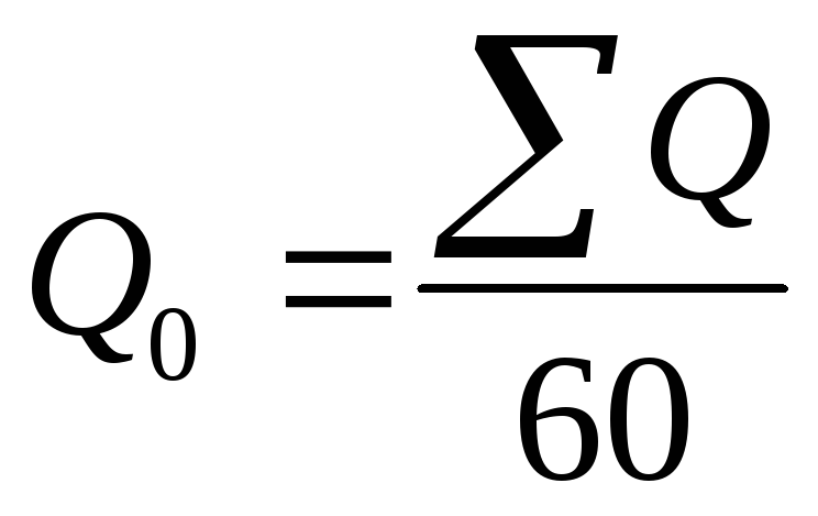 ,
,
модульные коэффициенты расходов
убывающего ряда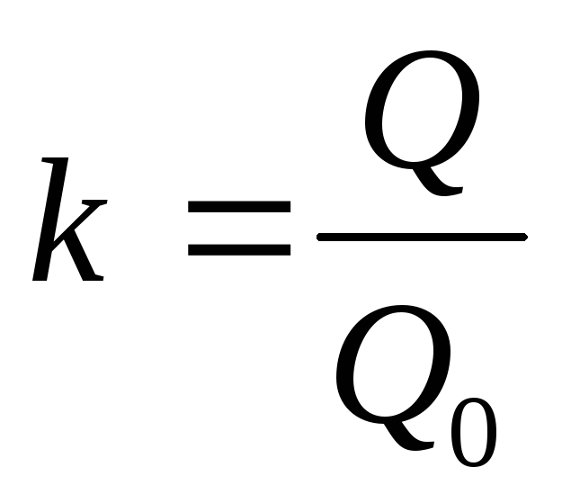 (гр. 5) и значения (k
-1), (k -1)2,
(k -1)3 (гр. 6 —
9). Вычисления выполняются с точностьюk – два знака после
запятой,
(k
-1)2, (k -1)3– четыре знака после запятой.
Контроль
вычислений
 (числу членов ряда);
 .Погрешности
за счет округления k
при
вычислении его с помощью логарифмической
линейки обычно не велики, и если невязка
не превышает 0,2—0,4, то она разбрасывается
в ряд k.
Грубые
ошибки вычисления k
и
(k—1)2
скажутся на
точности Cv
и
кривой обеспеченности, и поэтому значения
k
должны
быть исправлены.
Значения
Cv
и
Ся
вычисляются по алгебраическим суммам
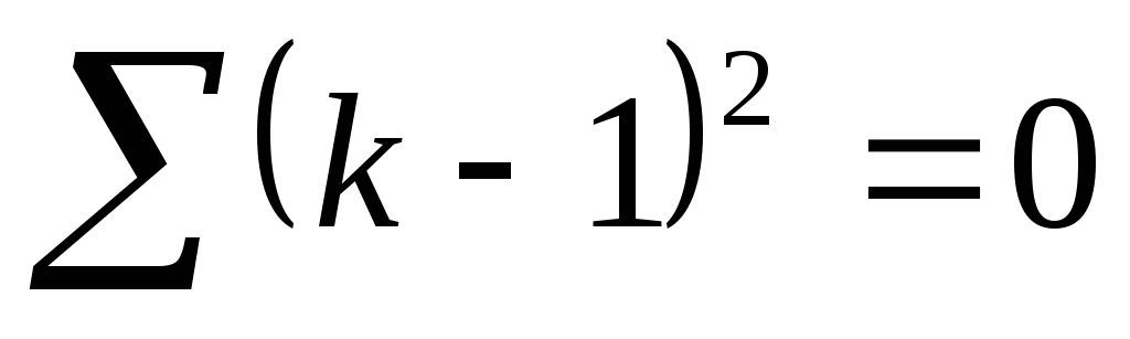
и
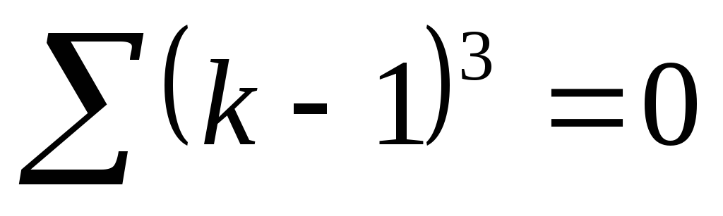 .
.
Таблица
3.11.
Подсчет коэффициента
вариации и асимметрии годового стока
р. Енисея
у г. Енисейска
F=
1420 000 км2
|
№ пп |
Год |
Q м3/сек |
Q,
в убывающем |
k |
(k |
(k |
(k-1)3 |
р, % |
||
|
+ |
|
+ |
|
|||||||
|
1 |
2 |
3 |
4 |
5 |
6 |
7 |
8 |
9 |
10 |
11 |
|
1 |
1903 |
6560 |
10200 |
1,34 |
0,34 |
0,1156 |
0,0393 |
1,64 |
||
|
2 |
1904 |
8100 |
9350 |
1,22 |
0,22 |
0,0484 |
0,0106 |
3,28 |
||
|
3 |
1905 |
7350 |
9260 |
1,21 |
0,21 |
0,0441 |
0,0093 |
4,92 |
||
|
… |
||||||||||
|
56 |
1962 |
6680 |
6610 |
0,86 |
0,14 |
0,0196 |
0,0027 |
91,8 |
||
|
57 |
1963 |
6950 |
6660 |
0,86 |
0,14 |
0,0196 |
0,0027 |
93,5 |
||
|
58 |
1964 |
6400 |
6420 |
0,84 |
0,16 |
0,0256 |
0,0041 |
95,1 |
||
|
59 |
1965 |
7360 |
6400 |
0,84 |
0,16 |
0,0256 |
0,0041 |
96,9 |
||
|
60 |
1966 |
8480 |
6180 |
0,81 |
0,19 |
0,0361 |
0,0069 |
98,5 |
||
|
Сумма |
59,96 |
0 |
0,6944 |
0,0458 |
Q0=7640
м3/сек
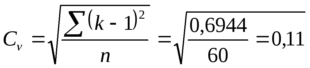 ;
;
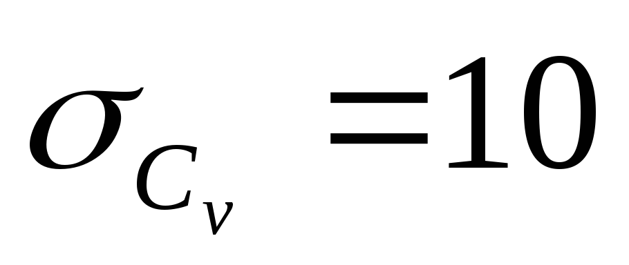 %
%
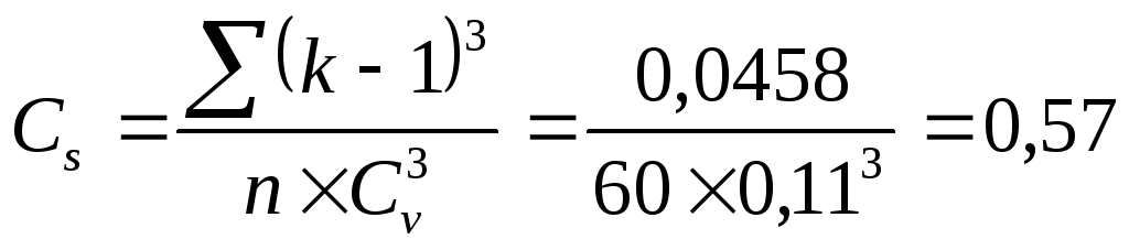 ;
;
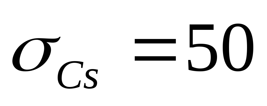 %
%
Параметры кривой
обеспеченности годового стока р. Енисея
у г. Енисейска, вычисленные по 60-летнему
ряду наблюдений, и их средние квадратические
ошибки , Q0= 7640 м3/сек,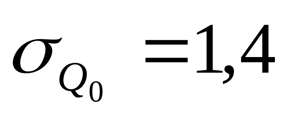 %,Cv
%,Cv
= 0,11,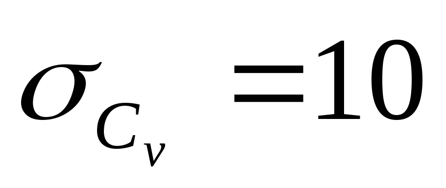 %,Сs=0,57,
 %.
%.
Ошибки определения
Q0
и Cv
незначительны, и вычисленные значения
Qo
и Си могут быть приняты
для дальнейших расчетов. Ошибка Cs
при n
= 60 годам получилась
большой. Поэтому расчетную кривую
обеспеченности выбираем из двух
теоретических кривых, построенных при
Cs
вычисленном и Cs
= 2 Cv.
Кривые обеспеченности построим для
расходов.
Сначала
строим эмпирическую кривую обеспеченности.
Для этого пользуемся графами 5 и 11 табл.
3.11.
Построение выполняем на специальной
клетчатке (см. рис. 3.1).
Затем вычисляем ординаты теоретических
кривых обеспеченности. Так как Cv
=0,11, то для построения теоретических
кривых обеспеченности пользуемся
таблицами биномиальной кривой (приложение
6 и 7). Вычисления ординат кривой при Cs
= 0,57 сводятся в табл. 3.12.
Значения ФР
выписываем из строчки
приложения 6, соответствующей Cs=0,57.
Значения kp
и Qp.
При
CS=2CV
пользуемся таблицей ординат кривой
обеспеченности (приложение 7), где
приводятся значения kp,
соответствующие Cv
(значения kp
выписываем из строки
Cv
= 0,11). По вычисленным QP
построены две теоретические кривые
обеспеченности, совмещенные с эмпирической
кривой (рис. 1).
Сопоставление
совмещенных кривых позволяет сделать
вывод, что теоретическая кривая
обеспеченности, построенная при Cs=0,57,
лучше соответствует эмпирической кривой
(наблюденным точкам) во всем диапазоне
и поэтому она принимается в качестве
расчетной (табл. 3.13).
Таблица
3.12.
Вычисление
ординат кривой обеспеченности годовых
расходов воды р. Енисея у г. Енисейска
N= 60,Q0= 7640 м3/сек,Cv
= 0,11
|
р, |
0,1 |
1 |
5 |
10 |
25 |
50 |
75 |
80 |
90 |
95 |
97 |
99 |
99,9 |
|
Сs=0,57 |
|||||||||||||
|
Фр |
3,92 |
2,73 |
1,79 |
1,32 |
0,62 |
-0,1 |
-0,72 |
-1,85 |
-1,2 |
-1,46 |
-1,63 |
-1,9 |
-2,3 |
|
Фр |
0,43 |
0,3 |
0,2 |
0,14 |
0,07 |
-0,01 |
-0,08 |
-0,09 |
-0,13 |
-0,16 |
-0,18 |
-0,21 |
-0,25 |
|
kp |
1,43 |
1,3 |
1,2 |
1,14 |
1,07 |
0,99 |
0,92 |
0,91 |
0,87 |
0,84 |
0,82 |
0,79 |
0,75 |
|
Qp |
10900 |
9940 |
9140 |
8640 |
8170 |
7560 |
7020 |
6950 |
6630 |
6420 |
6250 |
6020 |
5720 |
|
Сs |
|||||||||||||
|
kp |
1,37 |
1,27 |
1,19 |
1,14 |
1,07 |
1,0 |
0,92 |
0,91 |
0,86 |
0,83 |
0,80 |
0,76 |
0,70 |
|
Qp |
10530 |
9700 |
9090 |
8700 |
8170 |
7640 |
7020 |
6950 |
6560 |
6340 |
6100 |
5800 |
5340 |
Таблица
3.13.
Годовые расходы
воды р. Енисея у г. Енисейска заданных
обеспеченностей
Qo
= 7640 м3/сек,
и Cv
= 0,11, Cs=0,57.
|
Обеспеченность |
5 |
10 |
50 |
75 |
90 |
95 |
97 |
99 |
|
Qp |
9140 |
8640 |
7560 |
7020 |
6630 |
6420 |
6250 |
6020 |

Рис.3.1.
Кривые обеспеченности средних годовых
расходов воды р. Енисея у г. Енисейска,
n
=60, Q0=7640
м*/сек, Cv
= 0,11, Cs=0,57.
Пример
3.2.
Определить
параметры кривой обеспеченностей
и значения годового стока разной
обеспеченности р. Илека (F=
11 000 км2)
р=5, 10, 25, 50, 75, 95, 97 и 99%.
Для решения
поставленной задачи необходимо:
-
вычислить
параметры кривой обеспеченности Q0,
Cv
и
Cs; -
построить кривые
обеспеченности – эмпирическую и
теоретическую;
-
по
принятой теоретической кривой
обеспеченности вычислить расходы воды
заданной обеспеченности.
Cv
и
Са
вычисляются
методом моментов.
-
№
Год
Мср, л/сек
с 1 км21
1940
0,72
2
1941
3,39
3
1942
5,19
4
1944
0,43
5
1946
4,04
6
1947
1,23
7
1948
3,75
8
1949
2,54
9
1950
0,70
10
1951
0,68
11
1952
2,74
12
1953
0,95
13
1954
1,25
14
1955
0,78
15
1956
1,16
16
1957
3,74
17
1958
1,64
18
1959
1,50
19
1960
1,79
20
1961
0,82
21
1962
1,06
Содержание курса лекций «Статистика»
Показатели вариации в анализе взаимосвязей

Для измерения степени колеблемости отдельных значений признака относительно средней исчисляют основные показатели вариации.
Информация о средних уровнях исследуемых показателей обычно бывает недостаточной для полного анализа изучаемого процесса или явления. Иногда совершенно непохожие по своему внутреннему строению совокупности могут иметь равные средние величины. Поэтому для более детального изучения того или иного явления необходимо учитывать разброс или вариацию значений отдельных единиц совокупности. Измерение вариации признаков имеет как теоретическое, так и практическое значение.
Так, например, для выявления наиболее стабильно работающего коллектива или предприятия наравне с другими показателями рассчитывают и основные показатели вариации. Эти показатели дают возможность количественно определить размеры устойчивости производительности труда, уровня квалификации, цен на основные виды выпускаемой продукции и т.п. Измерение размеров вариации такого показателя, как «выполнение работ в срок» имеет важное значение для принятия решений заказчиками и инвесторами, т.к. ситуация, в которой присутствует изменчивость признака, часто содержит риск. Особое значение показатели вариации приобретают в анализе рынка ценных бумаг, где мера колеблемости отождествляется с мерой рискованности вложения денежных средств.
Основными показателями, характеризующими вариацию, являются:
- размах вариации;
- среднее линейное отклонение;
- дисперсия;
- среднее квадратическое отклонение;
- коэффициент вариации.
1) Размах вариации

(9.1 ) – размах вариации
2) Среднее линейное отклонение исчисляют для того, чтобы дать обобщающую характеристику распределению отклонений:

(9.2) – среднее линейное отклонение для несгруппированных данных

(9.3) – среднее линейное отклонение для вариационного ряда
где – абсолютные значения отклонений отдельных вариантов xi от средней арифметической ; fi – частота.
3. Дисперсия – это средняя арифметическая квадратов отклонений отдельных значений признака от их средней арифметической:

(9.4) – дисперсия
4. Среднее квадратическое отклонение – корень квадратный из дисперсии:

(9.5) – среднее квадратическое отклонение для несгруппированных данных

(9.6)- среднее квадратическое отклонение для вариационного ряда
!!!В отличие от дисперсии среднее квадратическое отклонение является абсолютной мерой вариации признака в совокупности и выражается в единицах измерения варьирующего признака (руб., тыс., млн и т.д.).!!!
5. Коэффициент вариации – используется для сравнительной оценки вариации, а также для характеристики однородности совокупности:

(9.7) – коэффициент вариации
Пример. Для иллюстрации расчетов воспользуемся данными нижеприведенной табл. 9.1:
Таблица 9.1 ‑ Данные о продаже основных марок холодильников:
| Модель | Цена
( $ ) |
Объем продаж (шт.) | xifi | |
| 1 | Siemens | 1000 | 30 | 30000 |
| 2 | Bosch | 800 | 26 | 20800 |
| 3 | AEG Santo | 900 | 24 | 21600 |
| 4 | Miele KF | 1200 | 30 | 36000 |
| 5 | Gorenje | 870 | 20 | 17400 |
| 6 | Haier | 570 | 23 | 13110 |
| 7 | Samsung | 760 | 30 | 22800 |
| 8 | Zanussi | 700 | 20 | 14000 |
| 9 | Daewoo | 460 | 20 | 9200 |
| 10 | Beko | 650 | 25 | 16250 |
| 11 | Candy | 480 | 20 | 9600 |
| 10 | Whirpool | 470 | 21 | 9870 |
| ИТОГО | 8860 | 289 | 220630 |
Рассчитаем размах вариации.
R= 1200-460=740$
Пример вычисления размаха вариации
Размах вариации служит незаменимой мерой разброса экстремальных значений признака. Кроме характеристики границ разброса признака, размах вариации может быть использован для выявления ошибок. При наличии очень больших (или очень малых) ошибочно записанных значений признака размах вариации сразу резко возрастает, что требует проверки и корректировки исходных данных.
Недостатком данного показателя является то, что он оценивает только границы варьирующего признака и не отражает его колеблемость внутри этих границ. Вследствие этого размах вариации может неправильно характеризовать общую колеблемость признака.
Этого недостатка лишен другой показатель – дисперсия, рассчитываемый как средний квадрат отклонений значений признака от их средней величины.
Между индивидуальными отклонениями от средней и колеблемостью признака существует прямая зависимость: чем сильнее колеблемость признака, тем больше отклонения его значений от средней величины и менее устойчив изучаемый показатель.
Как и средняя величина этот показатель может быть рассчитан в двух формах: взвешенной и невзвешенной
По приведенным выше данным определим средневзвешенную цену холодильника:

Пример вычисления средней арифметической взвешенной
Далее рассчитаем дисперсию:

Пример вычисления дисперсии
!!!Следует отметить, что дисперсия еще не дает представления об однородности совокупности, и этому показателю трудно дать экономическую интерпретацию, т.к. он рассчитан в квадратных единицах. Поэтому следующим шагом в исследовании однородности совокупности является расчет среднего квадратического отклонения, показывающего, насколько в среднем отклоняются конкретные варианты признака от его среднего значения. Оно определяется как квадратный корень из дисперсии и имеет ту же размерность что и изучаемый признак.!!!
Рассчитаем среднее квадратическое отклонение

Пример вычисления среднего квадратического отклонения
Вывод: Таким образом, цена каждой марки холодильника отклоняется от средней цены в среднем на 271,1 $
Рассмотренные показатели позволяют получить абсолютное значение вариации признака. Однако для сравнения разных совокупностей с точки зрения устойчивости какого-либо одного признака или для определения однородности совокупности рассчитывают относительные показатели.
Эти показатели вычисляются как отношение размаха вариации, среднего линейного отклонения или среднего квадратического отклонения к средней арифметической или медиане. Чаще всего эти показатели выражаются в процентах.
Определим значение показателя вариации по вышеприведенным данным таблицы

Пример вычисления показателя вариации
Совокупность считается однородной, если V не превышает 33%.
Если V<10% вариация признака слабая;
10% < V<25% – вариация средняя;
V>25% – вариация сильная.
Вывод: Рассчитанная величина свидетельствует о неоднородности цен на холодильники, т.к. однородной совокупность считается, если коэффициент вариации меньше 33% (для распределений близких к нормальному).
!! Следует отметить, что коэффициент вариации может быть более 100%, что, в частности, может быть при наличии значений сильно отличающихся от средней величины. Такой результат означает, что в исследуемой совокупности сильна вариация признаков по отношению к средней величине.
Изучая вариацию интересующего нас признака в пределах исследуемой совокупности и опираясь на общую среднюю в расчетах, трудно оценить степень воздействия на него какого-либо отдельного признака.
При проведении такого анализа исходная совокупность должна представлять собой множество единиц, каждая из которых характеризуется двумя признаками – факторным (оказывающим влияние на взаимосвязанный с ним признак) и результативным (подверженным влиянию).
Для выявления взаимосвязи исходная совокупность делится по факторному признаку на группы. Выводы о степени взаимосвязи базируются на анализе вариации результативного признака. Если статистическая совокупность разбита на группы по какому-либо признаку, то для оценки влияния различных факторов, определяющих вариацию индивидуальных значений признака, используют правило сложения дисперсий.
Общая дисперсия представляет собой сумму средней из виутригрупповой и межгрупповой и дисперсий:

(9.8) – общая дисперсия
где:

Общая дисперсия характеризует вариацию признака по всей совокупности как результат влияния всех факторов, определяющих индивидуальные различия единиц совокупности.

(9.9)
где:

Межгрупповая дисперсия характеризует вариацию, обусловленную влиянием фактора, положенного в основу группировки.

(9.10) – межгрупповая дисперсия
где:

Средняя из внутригрупповых дисперсий отражает ту часть вариации результативного признака, которая обусловлена действием всех прочих неучтенных факторов, кроме фактора, по которому осуществлялась группировка. Другими словами внутригрупповая дисперсия отражает случайную вариацию. Внутригрупповая дисперсия рассчитывается отдельно по каждой j-ой группе.

(9.11) – внутригрупповая дисперсия
где:

Для всех групп в целом вычисляется средняя из внутригрупповых дисперсий, взвешенных на частоты соответствующих групп по формуле:

(9.12) – средняя из внутригрупповых дисперсий
Взаимосвязь между тремя видами дисперсий получила название правила сложения дисперсий. Таким образом, зная два вида дисперсий всегда можно определить третий:

(9.13) – правило сложения дисперсий
Из этого равенства следует, что общая дисперсия, как правило, будет больше средней из групповых дисперсий. Это обусловлено тем, что при расчленении общей совокупности единиц на части по какому-либо признаку образуются более или менее однородные группы, в результате чего сокращается колеблемость признаков в пределах каждой группы. Это приводит к тому, что средняя из групповых дисперсий оказывается меньше дисперсии признака по всей совокупности единиц, причем разница между этими показателями будет тем больше, чем однороднее получаются группы в результате расчленения общей совокупности.
Теснота связи между факторным и результативным признаками оценивается на основе эмпирического корреляционного отношения:

(9.14)
Данный показатель может принимать значения от 0 до 1. Чем ближе к 1 будет его величина, тем сильнее взаимосвязь между рассматриваемыми признаками.
Пример. На следующем условном примере исследуем зависимость объема выполненных работ от формы собственности проектно-изыскательских организаций.
Таблица 9.2. Выполнение работ проектно-изыскательскими организациями разной формы собственности
| Форма собственности | Количество предприятий |
Объем выполненных работ (млн. руб.) |
Итого |
| Государственная | 4 | 10,30,20,40 | 100 |
| Негосударственная | 6 | 20, 40, 60, 20, 50, 50 | 240 |
| Итого | 10 | 340 |
Решение:
1) Определим средний объем работ для предприятий двух форм собственности.

2) Определим средний объем работ для каждой формы собственности.

3) Рассчитаем общую и внутригрупповые (т.е. для каждой группы) дисперсии.

4) Определим среднюю из внутригрупповых и межгрупповую дисперсию. Для этого полученные ранее данные заносятся в таблицу расчета.
Таблица 9.3. – Вспомогательная таблица
|
Форма собственности |
Число предприятий |
Средняя
по группе |
Внутригрупповые дисперсии |
| Государственная | 4 | 25 | 125 |
| Негосударственная | 6 | 40 | 233 |
| Итого | 10 |
Пример. Средняя из внутригрупповых дисперсий

Пример. Межгрупповая дисперсия

На последнем этапе решения задачи необходимо проверить тождество, отражающее закон сложения дисперсий:
Проверка закона сложения дисперсий: 54,0+189,8=243,8
Вывод: Таким образом, можно сделать вывод о том, что объем работ, выполненных проектно-изыскательскими организациями на 22% [(54,0/243,8) х 100%] зависит от фактора, положенного в основание группировки, т.е. от формы собственности, а на 78% [(189,8/243,8)х100%)] ‑ от прочих факторов.
Вывод о том, что объем выполненных работ в гораздо большей степени зависит от каких-либо других факторов, чем от формы собственности предприятий подтверждается и величиной эмпирического корреляционного отношения:

Вывод: Величина этого показателя свидетельствует о том, что зависимость объема работ от формы собственности предприятия невелика
Содержание курса лекций «Статистика»
Контрольные задания
- Распределение студентов одного из факультетов по возрасту характеризуется следующими данными:
| Возраст студентов, лет | 17 | 18 | 19 | 20 | 21 | 22 | 23 | 24 | Всего |
| Число студентов | 20 | 80 | 90 | 110 | 130 | 170 | 90 | 60 | 750 |
Вычислить: а) размах вариации; б)среднее линейное отклонение; в) дисперсию; г) среднее квадратическое отклонение; относительные показатели вариации возраста студентов.
2. По данным статистических ежегодников постройте таблицу с рядом показателей и определите показатели вариации: а) размах; б) среднее линейное отклонение; в) среднее квадратическое отклонение; г) коэффициент вариации. Оцените количественную однородность совокупности.
Содержание курса лекций «Статистика»
From Wikipedia, the free encyclopedia
In probability theory and statistics, the coefficient of variation (CV), also known as relative standard deviation (RSD),[citation needed] is a standardized measure of dispersion of a probability distribution or frequency distribution. It is often expressed as a percentage, and is defined as the ratio of the standard deviation 


Definition[edit]
The coefficient of variation (CV) is defined as the ratio of the standard deviation 


It shows the extent of variability in relation to the mean of the population.
The coefficient of variation should be computed only for data measured on scales that have a meaningful zero (ratio scale) and hence allow relative comparison of two measurements (i.e., division of one measurement by the other). The coefficient of variation may not have any meaning for data on an interval scale.[2] For example, most temperature scales (e.g., Celsius, Fahrenheit etc.) are interval scales with arbitrary zeros, so the computed coefficient of variation would be different depending on the scale used. On the other hand, Kelvin temperature has a meaningful zero, the complete absence of thermal energy, and thus is a ratio scale. In plain language, it is meaningful to say that 20 Kelvin is twice as hot as 10 Kelvin, but only in this scale with a true absolute zero. While a standard deviation (SD) can be measured in Kelvin, Celsius, or Fahrenheit, the value computed is only applicable to that scale. Only the Kelvin scale can be used to compute a valid coefficient of variability.
Measurements that are log-normally distributed exhibit stationary CV; in contrast, SD varies depending upon the expected value of measurements.
A more robust possibility is the quartile coefficient of dispersion, half the interquartile range 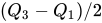
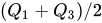
In most cases, a CV is computed for a single independent variable (e.g., a single factory product) with numerous, repeated measures of a dependent variable (e.g., error in the production process). However, data that are linear or even logarithmically non-linear and include a continuous range for the independent variable with sparse measurements across each value (e.g., scatter-plot) may be amenable to single CV calculation using a maximum-likelihood estimation approach.[3]
Examples[edit]
In the examples below, we will take the values given as randomly chosen from a larger population of values.
- The data set [100, 100, 100] has constant values. Its standard deviation is 0 and average is 100, giving the coefficient of variation as 0 / 100 = 0
- The data set [90, 100, 110] has more variability. Its standard deviation is 10 and its average is 100, giving the coefficient of variation as 10 / 100 = 0.1
- The data set [1, 5, 6, 8, 10, 40, 65, 88] has still more variability. Its standard deviation is 32.9 and its average is 27.9, giving a coefficient of variation of 32.9 / 27.9 = 1.18
In these examples, we will take the values given as the entire population of values.
- The data set [100, 100, 100] has a population standard deviation of 0 and a coefficient of variation of 0 / 100 = 0
- The data set [90, 100, 110] has a population standard deviation of 8.16 and a coefficient of variation of 8.16 / 100 = 0.0816
- The data set [1, 5, 6, 8, 10, 40, 65, 88] has a population standard deviation of 30.8 and a coefficient of variation of 30.8 / 27.9 = 1.10
Estimation[edit]
When only a sample of data from a population is available, the population CV can be estimated using the ratio of the sample standard deviation 


But this estimator, when applied to a small or moderately sized sample, tends to be too low: it is a biased estimator. For normally distributed data, an unbiased estimator[4] for a sample of size n is:
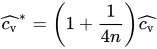
Log-normal data[edit]
In many applications, it can be assumed that data are log-normally distributed (evidenced by the presence of skewness in the sampled data).[5] In such cases, a more accurate estimate, derived from the properties of the log-normal distribution,[6][7][8] is defined as:
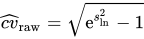
where 

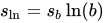


This term was intended to be analogous to the coefficient of variation, for describing multiplicative variation in log-normal data, but this definition of GCV has no theoretical basis as an estimate of 
For many practical purposes (such as sample size determination and calculation of confidence intervals) it is 
Comparison to standard deviation[edit]
Advantages[edit]
The coefficient of variation is useful because the standard deviation of data must always be understood in the context of the mean of the data.
In contrast, the actual value of the CV is independent of the unit in which the measurement has been taken, so it is a dimensionless number.
For comparison between data sets with different units or widely different means, one should use the coefficient of variation instead of the standard deviation.
Disadvantages[edit]
- When the mean value is close to zero, the coefficient of variation will approach infinity and is therefore sensitive to small changes in the mean. This is often the case if the values do not originate from a ratio scale.
- Unlike the standard deviation, it cannot be used directly to construct confidence intervals for the mean.
- CVs are not an ideal index of the certainty of measurement when the number of replicates varies across samples because CV is invariant to the number of replicates while the certainty of the mean improves with increasing replicates. In this case, standard error in percent is suggested to be superior.[13]
Applications[edit]
The coefficient of variation is also common in applied probability fields such as renewal theory, queueing theory, and reliability theory. In these fields, the exponential distribution is often more important than the normal distribution.
The standard deviation of an exponential distribution is equal to its mean, so its coefficient of variation is equal to 1. Distributions with CV < 1 (such as an Erlang distribution) are considered low-variance, while those with CV > 1 (such as a hyper-exponential distribution) are considered high-variance[citation needed]. Some formulas in these fields are expressed using the squared coefficient of variation, often abbreviated SCV. In modeling, a variation of the CV is the CV(RMSD). Essentially the CV(RMSD) replaces the standard deviation term with the Root Mean Square Deviation (RMSD). While many natural processes indeed show a correlation between the average value and the amount of variation around it, accurate sensor devices need to be designed in such a way that the coefficient of variation is close to zero, i.e., yielding a constant absolute error over their working range.
In actuarial science, the CV is known as unitized risk.[14]
In Industrial Solids Processing, CV is particularly important to measure the degree of homogeneity of a powder mixture. Comparing the calculated CV to a specification will allow to define if a sufficient degree of mixing has been reached.[15]
Laboratory measures of intra-assay and inter-assay CVs[edit]
CV measures are often used as quality controls for quantitative laboratory assays. While intra-assay and inter-assay CVs might be assumed to be calculated by simply averaging CV values across CV values for multiple samples within one assay or by averaging multiple inter-assay CV estimates, it has been suggested that these practices are incorrect and that a more complex computational process is required.[16] It has also been noted that CV values are not an ideal index of the certainty of a measurement when the number of replicates varies across samples − in this case standard error in percent is suggested to be superior.[13] If measurements do not have a natural zero point then the CV is not a valid measurement and alternative measures such as the intraclass correlation coefficient are recommended.[17]
As a measure of economic inequality[edit]
The coefficient of variation fulfills the requirements for a measure of economic inequality.[18][19][20] If x (with entries xi) is a list of the values of an economic indicator (e.g. wealth), with xi being the wealth of agent i, then the following requirements are met:
- Anonymity – cv is independent of the ordering of the list x. This follows from the fact that the variance and mean are independent of the ordering of x.
- Scale invariance: cv(x) = cv(αx) where α is a real number.[20]
- Population independence – If {x,x} is the list x appended to itself, then cv({x,x}) = cv(x). This follows from the fact that the variance and mean both obey this principle.
- Pigou–Dalton transfer principle: when wealth is transferred from a wealthier agent i to a poorer agent j (i.e. xi > xj) without altering their rank, then cv decreases and vice versa.[20]
cv assumes its minimum value of zero for complete equality (all xi are equal).[20] Its most notable drawback is that it is not bounded from above, so it cannot be normalized to be within a fixed range (e.g. like the Gini coefficient which is constrained to be between 0 and 1).[20] It is, however, more mathematically tractable than the Gini coefficient.
As a measure of standardisation of archaeological artefacts[edit]
Archaeologists often use CV values to compare the degree of standardisation of ancient artefacts.[21][22] Variation in CVs has been interpreted to indicate different cultural transmission contexts for the adoption of new technologies.[23] Coefficients of variation have also been used to investigate pottery standardisation relating to changes in social organisation.[24] Archaeologists also use several methods for comparing CV values, for example the modified signed-likelihood ratio (MSLR) test for equality of CVs.[25][26]
Examples of misuse[edit]
Comparing coefficients of variation between parameters using relative units can result in differences that may not be real. If we compare the same set of temperatures in Celsius and Fahrenheit (both relative units, where kelvin and Rankine scale are their associated absolute values):
Celsius: [0, 10, 20, 30, 40]
Fahrenheit: [32, 50, 68, 86, 104]
The sample standard deviations are 15.81 and 28.46, respectively. The CV of the first set is 15.81/20 = 79%. For the second set (which are the same temperatures) it is 28.46/68 = 42%.
If, for example, the data sets are temperature readings from two different sensors (a Celsius sensor and a Fahrenheit sensor) and you want to know which sensor is better by picking the one with the least variance, then you will be misled if you use CV. The problem here is that you have divided by a relative value rather than an absolute.
Comparing the same data set, now in absolute units:
Kelvin: [273.15, 283.15, 293.15, 303.15, 313.15]
Rankine: [491.67, 509.67, 527.67, 545.67, 563.67]
The sample standard deviations are still 15.81 and 28.46, respectively, because the standard deviation is not affected by a constant offset. The coefficients of variation, however, are now both equal to 5.39%.
Mathematically speaking, the coefficient of variation is not entirely linear. That is, for a random variable 


Distribution[edit]
Provided that negative and small positive values of the sample mean occur with negligible frequency, the probability distribution of the coefficient of variation for a sample of size 

where the symbol 


This is useful, for instance, in the construction of hypothesis tests or confidence intervals.
Statistical inference for the coefficient of variation in normally distributed data is often based on McKay’s chi-square approximation for the coefficient of variation [28][29][30][31][32][33]
Alternative[edit]
According to Liu (2012),[34]
Lehmann (1986).[35] «also derived the sample distribution of CV in order to give an exact method for the construction of a confidence interval for CV;» it is based on a non-central t-distribution.[incomprehensible]
Similar ratios[edit]
Standardized moments are similar ratios, 


In signal processing, particularly image processing, the reciprocal ratio 
Other related ratios include:
See also[edit]
- Omega ratio
- Sampling (statistics)
- Sharpe ratio
- Variance function
References[edit]
- ^ Everitt, Brian (1998). The Cambridge Dictionary of Statistics. Cambridge, UK New York: Cambridge University Press. ISBN 978-0521593465.
- ^ «What is the difference between ordinal, interval and ratio variables? Why should I care?». GraphPad Software Inc. Archived from the original on 15 December 2008. Retrieved 22 February 2008.
- ^ Odic, Darko; Im, Hee Yeon; Eisinger, Robert; Ly, Ryan; Halberda, Justin (June 2016). «PsiMLE: A maximum-likelihood estimation approach to estimating psychophysical scaling and variability more reliably, efficiently, and flexibly». Behavior Research Methods. 48 (2): 445–462. doi:10.3758/s13428-015-0600-5. ISSN 1554-3528. PMID 25987306.
- ^ Sokal RR & Rohlf FJ. Biometry (3rd Ed). New York: Freeman, 1995. p. 58. ISBN 0-7167-2411-1
- ^ Limpert, Eckhard; Stahel, Werner A.; Abbt, Markus (2001). «Log-normal Distributions across the Sciences: Keys and Clues». BioScience. 51 (5): 341–352. doi:10.1641/0006-3568(2001)051[0341:LNDATS]2.0.CO;2.
- ^ Koopmans, L. H.; Owen, D. B.; Rosenblatt, J. I. (1964). «Confidence intervals for the coefficient of variation for the normal and log normal distributions». Biometrika. 51 (1–2): 25–32. doi:10.1093/biomet/51.1-2.25.
- ^ Diletti, E; Hauschke, D; Steinijans, VW (1992). «Sample size determination for bioequivalence assessment by means of confidence intervals». International Journal of Clinical Pharmacology, Therapy, and Toxicology. 30 Suppl 1: S51–8. PMID 1601532.
- ^ Julious, Steven A.; Debarnot, Camille A. M. (2000). «Why Are Pharmacokinetic Data Summarized by Arithmetic Means?». Journal of Biopharmaceutical Statistics. 10 (1): 55–71. doi:10.1081/BIP-100101013. PMID 10709801. S2CID 2805094.
- ^ Reed, JF; Lynn, F; Meade, BD (2002). «Use of Coefficient of Variation in Assessing Variability of Quantitative Assays». Clin Diagn Lab Immunol. 9 (6): 1235–1239. doi:10.1128/CDLI.9.6.1235-1239.2002. PMC 130103. PMID 12414755.
- ^ Sawant,S.; Mohan, N. (2011) «FAQ: Issues with Efficacy Analysis of Clinical Trial Data Using SAS» Archived 24 August 2011 at the Wayback Machine, PharmaSUG2011, Paper PO08
- ^ Schiff, MH; et al. (2014). «Head-to-head, randomised, crossover study of oral versus subcutaneous methotrexate in patients with rheumatoid arthritis: drug-exposure limitations of oral methotrexate at doses >=15 mg may be overcome with subcutaneous administration». Ann Rheum Dis. 73 (8): 1–3. doi:10.1136/annrheumdis-2014-205228. PMC 4112421. PMID 24728329.
- ^ Kirkwood, TBL (1979). «Geometric means and measures of dispersion». Biometrics. 35 (4): 908–9. JSTOR 2530139.
- ^ a b Eisenberg, Dan (2015). «Improving qPCR telomere length assays: Controlling for well position effects increases statistical power». American Journal of Human Biology. 27 (4): 570–5. doi:10.1002/ajhb.22690. PMC 4478151. PMID 25757675.
- ^ Broverman, Samuel A. (2001). Actex study manual, Course 1, Examination of the Society of Actuaries, Exam 1 of the Casualty Actuarial Society (2001 ed.). Winsted, CT: Actex Publications. p. 104. ISBN 9781566983969. Retrieved 7 June 2014.
- ^ «Measuring Degree of Mixing — Homogeneity of powder mix — Mixture quality — PowderProcess.net». www.powderprocess.net. Archived from the original on 14 November 2017. Retrieved 2 May 2018.
- ^ Rodbard, D (October 1974). «Statistical quality control and routine data processing for radioimmunoassays and immunoradiometric assays». Clinical Chemistry. 20 (10): 1255–70. doi:10.1093/clinchem/20.10.1255. PMID 4370388.
- ^ Eisenberg, Dan T. A. (30 August 2016). «Telomere length measurement validity: the coefficient of variation is invalid and cannot be used to compare quantitative polymerase chain reaction and Southern blot telomere length measurement technique». International Journal of Epidemiology. 45 (4): 1295–1298. doi:10.1093/ije/dyw191. ISSN 0300-5771. PMID 27581804.
- ^ Champernowne, D. G.; Cowell, F. A. (1999). Economic Inequality and Income Distribution. Cambridge University Press.
- ^ Campano, F.; Salvatore, D. (2006). Income distribution. Oxford University Press.
- ^ a b c d e Bellu, Lorenzo Giovanni; Liberati, Paolo (2006). «Policy Impacts on Inequality – Simple Inequality Measures» (PDF). EASYPol, Analytical tools. Policy Support Service, Policy Assistance Division, FAO. Archived (PDF) from the original on 5 August 2016. Retrieved 13 June 2016.
- ^ Eerkens, Jelmer W.; Bettinger, Robert L. (July 2001). «Techniques for Assessing Standardization in Artifact Assemblages: Can We Scale Material Variability?». American Antiquity. 66 (3): 493–504. doi:10.2307/2694247. JSTOR 2694247. S2CID 163507589.
- ^ Roux, Valentine (2003). «Ceramic Standardization and Intensity of Production: Quantifying Degrees of Specialization». American Antiquity. 68 (4): 768–782. doi:10.2307/3557072. ISSN 0002-7316. JSTOR 3557072. S2CID 147444325.
- ^ Bettinger, Robert L.; Eerkens, Jelmer (April 1999). «Point Typologies, Cultural Transmission, and the Spread of Bow-and-Arrow Technology in the Prehistoric Great Basin». American Antiquity. 64 (2): 231–242. doi:10.2307/2694276. JSTOR 2694276. S2CID 163198451.
- ^ Wang, Li-Ying; Marwick, Ben (October 2020). «Standardization of ceramic shape: A case study of Iron Age pottery from northeastern Taiwan». Journal of Archaeological Science: Reports. 33: 102554. doi:10.1016/j.jasrep.2020.102554. S2CID 224904703.
- ^ Krishnamoorthy, K.; Lee, Meesook (February 2014). «Improved tests for the equality of normal coefficients of variation». Computational Statistics. 29 (1–2): 215–232. doi:10.1007/s00180-013-0445-2. S2CID 120898013.
- ^ Marwick, Ben; Krishnamoorthy, K (2019). cvequality: Tests for the equality of coefficients of variation from multiple groups. R package version 0.2.0.
- ^ Hendricks, Walter A.; Robey, Kate W. (1936). «The Sampling Distribution of the Coefficient of Variation». The Annals of Mathematical Statistics. 7 (3): 129–32. doi:10.1214/aoms/1177732503. JSTOR 2957564.
- ^ Iglevicz, Boris; Myers, Raymond (1970). «Comparisons of approximations to the percentage points of the sample coefficient of variation». Technometrics. 12 (1): 166–169. doi:10.2307/1267363. JSTOR 1267363.
- ^ Bennett, B. M. (1976). «On an approximate test for homogeneity of coefficients of variation». Contributions to Applied Statistics Dedicated to A. Linder. Experientia Supplementum. 22: 169–171. doi:10.1007/978-3-0348-5513-6_16. ISBN 978-3-0348-5515-0.
- ^ Vangel, Mark G. (1996). «Confidence intervals for a normal coefficient of variation». The American Statistician. 50 (1): 21–26. doi:10.1080/00031305.1996.10473537. JSTOR 2685039..
- ^ Feltz, Carol J; Miller, G. Edward (1996). «An asymptotic test for the equality of coefficients of variation from k populations». Statistics in Medicine. 15 (6): 647. doi:10.1002/(SICI)1097-0258(19960330)15:6<647::AID-SIM184>3.0.CO;2-P. PMID 8731006.
- ^ Forkman, Johannes (2009). «Estimator and tests for common coefficients of variation in normal distributions» (PDF). Communications in Statistics – Theory and Methods. 38 (2): 21–26. doi:10.1080/03610920802187448. S2CID 29168286. Archived (PDF) from the original on 6 December 2013. Retrieved 23 September 2013.
- ^ Krishnamoorthy, K; Lee, Meesook (2013). «Improved tests for the equality of normal coefficients of variation». Computational Statistics. 29 (1–2): 215–232. doi:10.1007/s00180-013-0445-2. S2CID 120898013.
- ^ Liu, Shuang (2012). Confidence Interval Estimation for Coefficient of Variation (Thesis). Georgia State University. p.3. Archived from the original on 1 March 2014. Retrieved 25 February 2014.
- ^ Lehmann, E. L. (1986). Testing Statistical Hypothesis. 2nd ed. New York: Wiley.
External links[edit]
- cvequality: R package to test for significant differences between multiple coefficients of variation
From Wikipedia, the free encyclopedia
In probability theory and statistics, the coefficient of variation (CV), also known as relative standard deviation (RSD),[citation needed] is a standardized measure of dispersion of a probability distribution or frequency distribution. It is often expressed as a percentage, and is defined as the ratio of the standard deviation
Definition[edit]
The coefficient of variation (CV) is defined as the ratio of the standard deviation
It shows the extent of variability in relation to the mean of the population.
The coefficient of variation should be computed only for data measured on scales that have a meaningful zero (ratio scale) and hence allow relative comparison of two measurements (i.e., division of one measurement by the other). The coefficient of variation may not have any meaning for data on an interval scale.[2] For example, most temperature scales (e.g., Celsius, Fahrenheit etc.) are interval scales with arbitrary zeros, so the computed coefficient of variation would be different depending on the scale used. On the other hand, Kelvin temperature has a meaningful zero, the complete absence of thermal energy, and thus is a ratio scale. In plain language, it is meaningful to say that 20 Kelvin is twice as hot as 10 Kelvin, but only in this scale with a true absolute zero. While a standard deviation (SD) can be measured in Kelvin, Celsius, or Fahrenheit, the value computed is only applicable to that scale. Only the Kelvin scale can be used to compute a valid coefficient of variability.
Measurements that are log-normally distributed exhibit stationary CV; in contrast, SD varies depending upon the expected value of measurements.
A more robust possibility is the quartile coefficient of dispersion, half the interquartile range
In most cases, a CV is computed for a single independent variable (e.g., a single factory product) with numerous, repeated measures of a dependent variable (e.g., error in the production process). However, data that are linear or even logarithmically non-linear and include a continuous range for the independent variable with sparse measurements across each value (e.g., scatter-plot) may be amenable to single CV calculation using a maximum-likelihood estimation approach.[3]
Examples[edit]
In the examples below, we will take the values given as randomly chosen from a larger population of values.
- The data set [100, 100, 100] has constant values. Its standard deviation is 0 and average is 100, giving the coefficient of variation as 0 / 100 = 0
- The data set [90, 100, 110] has more variability. Its standard deviation is 10 and its average is 100, giving the coefficient of variation as 10 / 100 = 0.1
- The data set [1, 5, 6, 8, 10, 40, 65, 88] has still more variability. Its standard deviation is 32.9 and its average is 27.9, giving a coefficient of variation of 32.9 / 27.9 = 1.18
In these examples, we will take the values given as the entire population of values.
- The data set [100, 100, 100] has a population standard deviation of 0 and a coefficient of variation of 0 / 100 = 0
- The data set [90, 100, 110] has a population standard deviation of 8.16 and a coefficient of variation of 8.16 / 100 = 0.0816
- The data set [1, 5, 6, 8, 10, 40, 65, 88] has a population standard deviation of 30.8 and a coefficient of variation of 30.8 / 27.9 = 1.10
Estimation[edit]
When only a sample of data from a population is available, the population CV can be estimated using the ratio of the sample standard deviation
But this estimator, when applied to a small or moderately sized sample, tends to be too low: it is a biased estimator. For normally distributed data, an unbiased estimator[4] for a sample of size n is:
Log-normal data[edit]
In many applications, it can be assumed that data are log-normally distributed (evidenced by the presence of skewness in the sampled data).[5] In such cases, a more accurate estimate, derived from the properties of the log-normal distribution,[6][7][8] is defined as:
where
This term was intended to be analogous to the coefficient of variation, for describing multiplicative variation in log-normal data, but this definition of GCV has no theoretical basis as an estimate of
For many practical purposes (such as sample size determination and calculation of confidence intervals) it is
Comparison to standard deviation[edit]
Advantages[edit]
The coefficient of variation is useful because the standard deviation of data must always be understood in the context of the mean of the data.
In contrast, the actual value of the CV is independent of the unit in which the measurement has been taken, so it is a dimensionless number.
For comparison between data sets with different units or widely different means, one should use the coefficient of variation instead of the standard deviation.
Disadvantages[edit]
- When the mean value is close to zero, the coefficient of variation will approach infinity and is therefore sensitive to small changes in the mean. This is often the case if the values do not originate from a ratio scale.
- Unlike the standard deviation, it cannot be used directly to construct confidence intervals for the mean.
- CVs are not an ideal index of the certainty of measurement when the number of replicates varies across samples because CV is invariant to the number of replicates while the certainty of the mean improves with increasing replicates. In this case, standard error in percent is suggested to be superior.[13]
Applications[edit]
The coefficient of variation is also common in applied probability fields such as renewal theory, queueing theory, and reliability theory. In these fields, the exponential distribution is often more important than the normal distribution.
The standard deviation of an exponential distribution is equal to its mean, so its coefficient of variation is equal to 1. Distributions with CV < 1 (such as an Erlang distribution) are considered low-variance, while those with CV > 1 (such as a hyper-exponential distribution) are considered high-variance[citation needed]. Some formulas in these fields are expressed using the squared coefficient of variation, often abbreviated SCV. In modeling, a variation of the CV is the CV(RMSD). Essentially the CV(RMSD) replaces the standard deviation term with the Root Mean Square Deviation (RMSD). While many natural processes indeed show a correlation between the average value and the amount of variation around it, accurate sensor devices need to be designed in such a way that the coefficient of variation is close to zero, i.e., yielding a constant absolute error over their working range.
In actuarial science, the CV is known as unitized risk.[14]
In Industrial Solids Processing, CV is particularly important to measure the degree of homogeneity of a powder mixture. Comparing the calculated CV to a specification will allow to define if a sufficient degree of mixing has been reached.[15]
Laboratory measures of intra-assay and inter-assay CVs[edit]
CV measures are often used as quality controls for quantitative laboratory assays. While intra-assay and inter-assay CVs might be assumed to be calculated by simply averaging CV values across CV values for multiple samples within one assay or by averaging multiple inter-assay CV estimates, it has been suggested that these practices are incorrect and that a more complex computational process is required.[16] It has also been noted that CV values are not an ideal index of the certainty of a measurement when the number of replicates varies across samples − in this case standard error in percent is suggested to be superior.[13] If measurements do not have a natural zero point then the CV is not a valid measurement and alternative measures such as the intraclass correlation coefficient are recommended.[17]
As a measure of economic inequality[edit]
The coefficient of variation fulfills the requirements for a measure of economic inequality.[18][19][20] If x (with entries xi) is a list of the values of an economic indicator (e.g. wealth), with xi being the wealth of agent i, then the following requirements are met:
- Anonymity – cv is independent of the ordering of the list x. This follows from the fact that the variance and mean are independent of the ordering of x.
- Scale invariance: cv(x) = cv(αx) where α is a real number.[20]
- Population independence – If {x,x} is the list x appended to itself, then cv({x,x}) = cv(x). This follows from the fact that the variance and mean both obey this principle.
- Pigou–Dalton transfer principle: when wealth is transferred from a wealthier agent i to a poorer agent j (i.e. xi > xj) without altering their rank, then cv decreases and vice versa.[20]
cv assumes its minimum value of zero for complete equality (all xi are equal).[20] Its most notable drawback is that it is not bounded from above, so it cannot be normalized to be within a fixed range (e.g. like the Gini coefficient which is constrained to be between 0 and 1).[20] It is, however, more mathematically tractable than the Gini coefficient.
As a measure of standardisation of archaeological artefacts[edit]
Archaeologists often use CV values to compare the degree of standardisation of ancient artefacts.[21][22] Variation in CVs has been interpreted to indicate different cultural transmission contexts for the adoption of new technologies.[23] Coefficients of variation have also been used to investigate pottery standardisation relating to changes in social organisation.[24] Archaeologists also use several methods for comparing CV values, for example the modified signed-likelihood ratio (MSLR) test for equality of CVs.[25][26]
Examples of misuse[edit]
Comparing coefficients of variation between parameters using relative units can result in differences that may not be real. If we compare the same set of temperatures in Celsius and Fahrenheit (both relative units, where kelvin and Rankine scale are their associated absolute values):
Celsius: [0, 10, 20, 30, 40]
Fahrenheit: [32, 50, 68, 86, 104]
The sample standard deviations are 15.81 and 28.46, respectively. The CV of the first set is 15.81/20 = 79%. For the second set (which are the same temperatures) it is 28.46/68 = 42%.
If, for example, the data sets are temperature readings from two different sensors (a Celsius sensor and a Fahrenheit sensor) and you want to know which sensor is better by picking the one with the least variance, then you will be misled if you use CV. The problem here is that you have divided by a relative value rather than an absolute.
Comparing the same data set, now in absolute units:
Kelvin: [273.15, 283.15, 293.15, 303.15, 313.15]
Rankine: [491.67, 509.67, 527.67, 545.67, 563.67]
The sample standard deviations are still 15.81 and 28.46, respectively, because the standard deviation is not affected by a constant offset. The coefficients of variation, however, are now both equal to 5.39%.
Mathematically speaking, the coefficient of variation is not entirely linear. That is, for a random variable
Distribution[edit]
Provided that negative and small positive values of the sample mean occur with negligible frequency, the probability distribution of the coefficient of variation for a sample of size
where the symbol
This is useful, for instance, in the construction of hypothesis tests or confidence intervals.
Statistical inference for the coefficient of variation in normally distributed data is often based on McKay’s chi-square approximation for the coefficient of variation [28][29][30][31][32][33]
Alternative[edit]
According to Liu (2012),[34]
Lehmann (1986).[35] «also derived the sample distribution of CV in order to give an exact method for the construction of a confidence interval for CV;» it is based on a non-central t-distribution.[incomprehensible]
Similar ratios[edit]
Standardized moments are similar ratios,
In signal processing, particularly image processing, the reciprocal ratio
Other related ratios include:
See also[edit]
- Omega ratio
- Sampling (statistics)
- Sharpe ratio
- Variance function
References[edit]
- ^ Everitt, Brian (1998). The Cambridge Dictionary of Statistics. Cambridge, UK New York: Cambridge University Press. ISBN 978-0521593465.
- ^ «What is the difference between ordinal, interval and ratio variables? Why should I care?». GraphPad Software Inc. Archived from the original on 15 December 2008. Retrieved 22 February 2008.
- ^ Odic, Darko; Im, Hee Yeon; Eisinger, Robert; Ly, Ryan; Halberda, Justin (June 2016). «PsiMLE: A maximum-likelihood estimation approach to estimating psychophysical scaling and variability more reliably, efficiently, and flexibly». Behavior Research Methods. 48 (2): 445–462. doi:10.3758/s13428-015-0600-5. ISSN 1554-3528. PMID 25987306.
- ^ Sokal RR & Rohlf FJ. Biometry (3rd Ed). New York: Freeman, 1995. p. 58. ISBN 0-7167-2411-1
- ^ Limpert, Eckhard; Stahel, Werner A.; Abbt, Markus (2001). «Log-normal Distributions across the Sciences: Keys and Clues». BioScience. 51 (5): 341–352. doi:10.1641/0006-3568(2001)051[0341:LNDATS]2.0.CO;2.
- ^ Koopmans, L. H.; Owen, D. B.; Rosenblatt, J. I. (1964). «Confidence intervals for the coefficient of variation for the normal and log normal distributions». Biometrika. 51 (1–2): 25–32. doi:10.1093/biomet/51.1-2.25.
- ^ Diletti, E; Hauschke, D; Steinijans, VW (1992). «Sample size determination for bioequivalence assessment by means of confidence intervals». International Journal of Clinical Pharmacology, Therapy, and Toxicology. 30 Suppl 1: S51–8. PMID 1601532.
- ^ Julious, Steven A.; Debarnot, Camille A. M. (2000). «Why Are Pharmacokinetic Data Summarized by Arithmetic Means?». Journal of Biopharmaceutical Statistics. 10 (1): 55–71. doi:10.1081/BIP-100101013. PMID 10709801. S2CID 2805094.
- ^ Reed, JF; Lynn, F; Meade, BD (2002). «Use of Coefficient of Variation in Assessing Variability of Quantitative Assays». Clin Diagn Lab Immunol. 9 (6): 1235–1239. doi:10.1128/CDLI.9.6.1235-1239.2002. PMC 130103. PMID 12414755.
- ^ Sawant,S.; Mohan, N. (2011) «FAQ: Issues with Efficacy Analysis of Clinical Trial Data Using SAS» Archived 24 August 2011 at the Wayback Machine, PharmaSUG2011, Paper PO08
- ^ Schiff, MH; et al. (2014). «Head-to-head, randomised, crossover study of oral versus subcutaneous methotrexate in patients with rheumatoid arthritis: drug-exposure limitations of oral methotrexate at doses >=15 mg may be overcome with subcutaneous administration». Ann Rheum Dis. 73 (8): 1–3. doi:10.1136/annrheumdis-2014-205228. PMC 4112421. PMID 24728329.
- ^ Kirkwood, TBL (1979). «Geometric means and measures of dispersion». Biometrics. 35 (4): 908–9. JSTOR 2530139.
- ^ a b Eisenberg, Dan (2015). «Improving qPCR telomere length assays: Controlling for well position effects increases statistical power». American Journal of Human Biology. 27 (4): 570–5. doi:10.1002/ajhb.22690. PMC 4478151. PMID 25757675.
- ^ Broverman, Samuel A. (2001). Actex study manual, Course 1, Examination of the Society of Actuaries, Exam 1 of the Casualty Actuarial Society (2001 ed.). Winsted, CT: Actex Publications. p. 104. ISBN 9781566983969. Retrieved 7 June 2014.
- ^ «Measuring Degree of Mixing — Homogeneity of powder mix — Mixture quality — PowderProcess.net». www.powderprocess.net. Archived from the original on 14 November 2017. Retrieved 2 May 2018.
- ^ Rodbard, D (October 1974). «Statistical quality control and routine data processing for radioimmunoassays and immunoradiometric assays». Clinical Chemistry. 20 (10): 1255–70. doi:10.1093/clinchem/20.10.1255. PMID 4370388.
- ^ Eisenberg, Dan T. A. (30 August 2016). «Telomere length measurement validity: the coefficient of variation is invalid and cannot be used to compare quantitative polymerase chain reaction and Southern blot telomere length measurement technique». International Journal of Epidemiology. 45 (4): 1295–1298. doi:10.1093/ije/dyw191. ISSN 0300-5771. PMID 27581804.
- ^ Champernowne, D. G.; Cowell, F. A. (1999). Economic Inequality and Income Distribution. Cambridge University Press.
- ^ Campano, F.; Salvatore, D. (2006). Income distribution. Oxford University Press.
- ^ a b c d e Bellu, Lorenzo Giovanni; Liberati, Paolo (2006). «Policy Impacts on Inequality – Simple Inequality Measures» (PDF). EASYPol, Analytical tools. Policy Support Service, Policy Assistance Division, FAO. Archived (PDF) from the original on 5 August 2016. Retrieved 13 June 2016.
- ^ Eerkens, Jelmer W.; Bettinger, Robert L. (July 2001). «Techniques for Assessing Standardization in Artifact Assemblages: Can We Scale Material Variability?». American Antiquity. 66 (3): 493–504. doi:10.2307/2694247. JSTOR 2694247. S2CID 163507589.
- ^ Roux, Valentine (2003). «Ceramic Standardization and Intensity of Production: Quantifying Degrees of Specialization». American Antiquity. 68 (4): 768–782. doi:10.2307/3557072. ISSN 0002-7316. JSTOR 3557072. S2CID 147444325.
- ^ Bettinger, Robert L.; Eerkens, Jelmer (April 1999). «Point Typologies, Cultural Transmission, and the Spread of Bow-and-Arrow Technology in the Prehistoric Great Basin». American Antiquity. 64 (2): 231–242. doi:10.2307/2694276. JSTOR 2694276. S2CID 163198451.
- ^ Wang, Li-Ying; Marwick, Ben (October 2020). «Standardization of ceramic shape: A case study of Iron Age pottery from northeastern Taiwan». Journal of Archaeological Science: Reports. 33: 102554. doi:10.1016/j.jasrep.2020.102554. S2CID 224904703.
- ^ Krishnamoorthy, K.; Lee, Meesook (February 2014). «Improved tests for the equality of normal coefficients of variation». Computational Statistics. 29 (1–2): 215–232. doi:10.1007/s00180-013-0445-2. S2CID 120898013.
- ^ Marwick, Ben; Krishnamoorthy, K (2019). cvequality: Tests for the equality of coefficients of variation from multiple groups. R package version 0.2.0.
- ^ Hendricks, Walter A.; Robey, Kate W. (1936). «The Sampling Distribution of the Coefficient of Variation». The Annals of Mathematical Statistics. 7 (3): 129–32. doi:10.1214/aoms/1177732503. JSTOR 2957564.
- ^ Iglevicz, Boris; Myers, Raymond (1970). «Comparisons of approximations to the percentage points of the sample coefficient of variation». Technometrics. 12 (1): 166–169. doi:10.2307/1267363. JSTOR 1267363.
- ^ Bennett, B. M. (1976). «On an approximate test for homogeneity of coefficients of variation». Contributions to Applied Statistics Dedicated to A. Linder. Experientia Supplementum. 22: 169–171. doi:10.1007/978-3-0348-5513-6_16. ISBN 978-3-0348-5515-0.
- ^ Vangel, Mark G. (1996). «Confidence intervals for a normal coefficient of variation». The American Statistician. 50 (1): 21–26. doi:10.1080/00031305.1996.10473537. JSTOR 2685039..
- ^ Feltz, Carol J; Miller, G. Edward (1996). «An asymptotic test for the equality of coefficients of variation from k populations». Statistics in Medicine. 15 (6): 647. doi:10.1002/(SICI)1097-0258(19960330)15:6<647::AID-SIM184>3.0.CO;2-P. PMID 8731006.
- ^ Forkman, Johannes (2009). «Estimator and tests for common coefficients of variation in normal distributions» (PDF). Communications in Statistics – Theory and Methods. 38 (2): 21–26. doi:10.1080/03610920802187448. S2CID 29168286. Archived (PDF) from the original on 6 December 2013. Retrieved 23 September 2013.
- ^ Krishnamoorthy, K; Lee, Meesook (2013). «Improved tests for the equality of normal coefficients of variation». Computational Statistics. 29 (1–2): 215–232. doi:10.1007/s00180-013-0445-2. S2CID 120898013.
- ^ Liu, Shuang (2012). Confidence Interval Estimation for Coefficient of Variation (Thesis). Georgia State University. p.3. Archived from the original on 1 March 2014. Retrieved 25 February 2014.
- ^ Lehmann, E. L. (1986). Testing Statistical Hypothesis. 2nd ed. New York: Wiley.
External links[edit]
- cvequality: R package to test for significant differences between multiple coefficients of variation