Относительная ошибка аппроксимации это

From Wikipedia, the free encyclopedia

For broader coverage of this topic, see Approximation.

Graph of $f(x)=e^{x}$ (blue) with its linear approximation $P_{1}(x)=1+x$ (red) at a = 0. The approximation error is the gap between the curves, and it increases for x values further from 0.

The approximation error in a data value is the discrepancy between an exact value and some approximation to it. This error can be expressed as an absolute error (the numerical amount of the discrepancy) or as a relative error (the absolute error divided by the data value).

An approximation error can occur because of computing machine precision or measurement error (e.g. the length of a piece of paper is 4.53 cm but the ruler only allows you to estimate it to the nearest 0.1 cm, so you measure it as 4.5 cm).

In the mathematical field of numerical analysis, the numerical stability of an algorithm indicates how the error is propagated by the algorithm.

Formal definition[edit]

One commonly distinguishes between the relative error and the absolute error.

Given some value v and its approximation v_approx, the absolute error is

$epsilon =|v-v_{text{approx}}| ,$

where the vertical bars denote the absolute value.
If $vneq 0,$ the relative error is

$eta ={frac {epsilon }{|v|}}=left|{frac {v-v_{text{approx}}}{v}}right|=left|1-{frac {v_{text{approx}}}{v}}right|,$

and the percent error (an expression of the relative error) is

${displaystyle delta =100%times eta =100%times {frac {epsilon }{|v|}}=100%times left|{frac {v-v_{text{approx}}}{v}}right|.}$

In words, the absolute error is the magnitude of the difference between the exact value and the approximation. The relative error is the absolute error divided by the magnitude of the exact value.

An error bound is an upper limit on the relative or absolute size of an approximation error.

Generalizations[edit]

These definitions can be extended to the case when $v$ and $v_{text{approx}}$ are n-dimensional vectors, by replacing the absolute value with an n-norm.^[1]

Examples[edit]

Best rational approximants for π (green circle), e (blue diamond), ϕ (pink oblong), (√3)/2 (grey hexagon), 1/√2 (red octagon) and 1/√3 (orange triangle) calculated from their continued fraction expansions, plotted as slopes y/x with errors from their true values (black dashes)

As an example, if the exact value is 50 and the approximation is 49.9, then the absolute error is 0.1 and the relative error is 0.1/50 = 0.002 = 0.2%. Another example would be if, in measuring a 6 mL beaker, the value read was 5 mL. The correct reading being 6 mL, this means the percent error in that particular situation is, rounded, 16.7%.

The relative error is often used to compare approximations of numbers of widely differing size; for example, approximating the number 1,000 with an absolute error of 3 is, in most applications, much worse than approximating the number 1,000,000 with an absolute error of 3; in the first case the relative error is 0.003 and in the second it is only 0.000003.

There are two features of relative error that should be kept in mind. Firstly, relative error is undefined when the true value is zero as it appears in the denominator (see below). Secondly, relative error only makes sense when measured on a ratio scale, (i.e. a scale which has a true meaningful zero), otherwise it would be sensitive to the measurement units. For example, when an absolute error in a temperature measurement given in Celsius scale is 1 °C, and the true value is 2 °C, the relative error is 0.5, and the percent error is 50%. For this same case, when the temperature is given in Kelvin scale, the same 1 K absolute error with the same true value of 275.15 K gives a relative error of 3.63×10⁻³ and a percent error of only 0.363%. Celsius temperature is measured on an interval scale, whereas the Kelvin scale has a true zero and so is a ratio scale. Thus the relative error is not very meaningful.

Instruments[edit]

In most indicating instruments, the accuracy is guaranteed to a certain percentage of full-scale reading. The limits of these deviations from the specified values are known as limiting errors or guarantee errors.^[2]

References[edit]

^ Golub, Gene; Charles F. Van Loan (1996). Matrix Computations – Third Edition. Baltimore: The Johns Hopkins University Press. p. 53. ISBN 0-8018-5413-X.
^ Helfrick, Albert D. (2005) Modern Electronic Instrumentation and Measurement Techniques. p. 16. ISBN 81-297-0731-4

External links[edit]

Weisstein, Eric W. «Percentage error». MathWorld.

Источник

From Wikipedia, the free encyclopedia

For broader coverage of this topic, see Approximation.

Graph of $f(x)=e^{x}$ (blue) with its linear approximation $P_{1}(x)=1+x$ (red) at a = 0. The approximation error is the gap between the curves, and it increases for x values further from 0.

In the mathematical field of numerical analysis, the numerical stability of an algorithm indicates how the error is propagated by the algorithm.

Formal definition[edit]

One commonly distinguishes between the relative error and the absolute error.

Given some value v and its approximation v_approx, the absolute error is

$epsilon =|v-v_{text{approx}}| ,$

where the vertical bars denote the absolute value.
If $vneq 0,$ the relative error is

$eta ={frac {epsilon }{|v|}}=left|{frac {v-v_{text{approx}}}{v}}right|=left|1-{frac {v_{text{approx}}}{v}}right|,$

and the percent error (an expression of the relative error) is

${displaystyle delta =100%times eta =100%times {frac {epsilon }{|v|}}=100%times left|{frac {v-v_{text{approx}}}{v}}right|.}$

In words, the absolute error is the magnitude of the difference between the exact value and the approximation. The relative error is the absolute error divided by the magnitude of the exact value.

An error bound is an upper limit on the relative or absolute size of an approximation error.

Generalizations[edit]

These definitions can be extended to the case when $v$ and $v_{text{approx}}$ are n-dimensional vectors, by replacing the absolute value with an n-norm.^[1]

Examples[edit]

Instruments[edit]

References[edit]

^ Golub, Gene; Charles F. Van Loan (1996). Matrix Computations – Third Edition. Baltimore: The Johns Hopkins University Press. p. 53. ISBN 0-8018-5413-X.
^ Helfrick, Albert D. (2005) Modern Electronic Instrumentation and Measurement Techniques. p. 16. ISBN 81-297-0731-4

External links[edit]

Weisstein, Eric W. «Percentage error». MathWorld.

Источник

Министерство
сельского хозяйства РФ

Федеральное
государственное бюджетное образовательное

учреждение
высшего профессионального образования

«Пермская
государственная сельскохозяйственная
академия

имени
академика Д.Н.Прянишникова»

Кафедра финансов,
кредита и экономического анализа

Выполнила:

студентка
3 курса заочного отделения

По
специальности: «Экономика и управление
на АПК»

Группа
ЭБУ-2011-1-4739

Гонцова
Елена Александровна

Проверил:
кандидат экономических наук Тупицина
Ольга Владимировна

Пермь 2014

Содержание

Ошибки
аппроксимации и ее определение………………………………….3
Аналитический
способ выравнивания временного ряда
и используемые при этом
функции……………………………………………………………..4
Практическая
часть…………………………………………………………..11
1. Задание
  1………………………………………………………………11
2. Задание
  2……………………………………………….………………19

Список
использованной литературы…………………………………………..25

Ошибки аппроксимации и ее определение.

Средняя ошибка
аппроксимации
– это среднее отклонение расчетных
данных от фактических. Она определяется
в процентах по модулю.

Фактические
значения результативного признака
отличаются от теоретических. Чем меньше
это отличие, тем ближе теоретические
значения подходят к эмпирическим данным,
это лучшее качество модели. Величина
отклонений фактических и расчетных
значений результативного признака по
каждому наблюдению представляет собой
ошибку аппроксимации. Их число
соответствует объему совокупности. В
отдельных случаях ошибка апроксимации
может оказаться равной нулю. Для сравнения
используются величины отклонений,
выраженные в процентах к фактическим
значениям.

Поскольку может
быть как величиной положительной, так
и отрицательной, то ошибки аппроксимации
для каждого наблюдения принято определять
в процентах по модулю. Отклонения можно
рассматривать как абсолютную ошибку
аппроксимации, и как относительную
ошибку аппроксимации. Чтоб иметь общее
суждение о качестве модели из относительных
отклонений по каждому наблюдению,
определяют среднюю ошибку аппроксимации
как среднюю арифметическую простую.

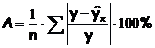
Среднюю ошибку
аппроксимации рассчитают по формуле:

Возможно и иное
определение средней ошибки аппроксимации:

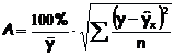
Если А£10-12%, то
можно говорить о хорошем качестве
модели.

Аналитический способ выравнивания временного ряда и используемые при этом функции.

Более
совершенным приемом выявления основной
тенденции развития в рядах динамики
является аналитическое выравнивание.
При изучении общей тенденции методом
аналитического выравнивания исходят
из того, что изменения уровней ряда
динамики могут быть с той или иной
степенью точности приближения выражены
определенными математическими функциями.
Вид уравнения определяется характером
динамики развития конкретного явления.
На практике по имеющемуся временному
ряду задают вид и находят параметры
функции y=f(t), а затем анализируют поведение
отклонений от тенденции. Чаще всего при
выравнивании используются следующие
зависимости: линейная, параболическая
и экспоненциальная. Во многих случаях
моделирование рядов динамики с помощью
полиномов или экспоненциальной функции
не дает удовлетворительных результатов,
так как в рядах динамики содержатся
заметные периодические колебания вокруг
общей тенденции. В таких случаях следует
использовать гармонический анализ
(гармоники ряда Фурье). Применение,
именно, этого метода предпочтительно,
поскольку он определяет закон, по
которому можно достаточно точно
спрогнозировать значения уровней ряда.

Целью же аналитического
выравнивания динамического ряда является
определение аналитической или графической
зависимости y=f(t). Функцию y=f(t) выбирают
таким образом, чтобы она давала
содержательное объяснение изучаемого
процесса. Это могут быть различные
функции.

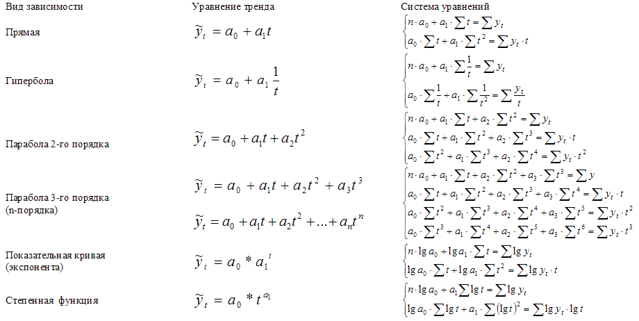
Системы уравнений
вида y=f(t) для оценки параметров полиномов
по МНК

(кликабельно)

Графическое
представление полиномов n-порядка

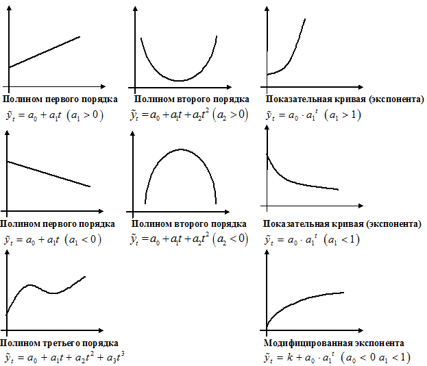
1.
Если изменение уровней ряда характеризуется
равномерным увеличением (уменьшением)
уровней, когда абсолютные цепные приросты
близки по величине, тенденцию развития
характеризует уравнение прямой линии.

2.
Если в результате анализа типа тенденции
динамики установлена криволинейная
зависимость, примерно с постоянным
ускорением, то форма тенденции выражается
уравнением параболы второго порядка.

3.
Если рост уровней ряда динамики происходит
в геометрической прогрессии, т.е. цепные
коэффициенты роста более или менее
постоянны, выравнивание ряда динамики
ведется по показательной функции.

После
выбора вида уравнения необходимо
определить параметры уравнения. Самый
распространенный способ определения
параметров уравнения — это метод
наименьших квадратов, в котором в
качестве решения принимается точка
минимума суммы квадратов отклонений
между теоретическими (выравненными по
выбранному уравнению) и эмпирическими
уровнями.

Выравнивание
по прямой (определение линии тренда)
имеет выражение: yt=a0+a1t

t—условное
обозначение времени;

а
0 и a1—параметры искомой прямой.

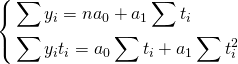
Параметры
прямой находятся из решения системы
уравнений:

Система уравнений
упрощается, если значения t подобрать
так, чтобы их сумма равнялась Σt = 0, т. е.
начало отсчета времени перенести в
середину рассматриваемого периода.
Если до переноса точки отсчета t = 1, 2, 3,
4…, то после переноса:

если число уровней
ряда нечетное t = -4 -3 -2 -1 0 +1 +2 +3 +4

если
число уровней ряда четное t = -7 -5 -3
-1 +1 +3 +5 +7

Таким образом, ∑t
в нечетной степени всегда будет равна
нулю.

Аналогично находятся
параметры параболы 2-го порядка из
решения системы уравнений:

Выравнивание
по среднему абсолютному приросту или
среднему коэффициенту роста:

Δ-средний абсолютный
прирост;

К-средний коэффициент
роста;

У0-начальный уровень
ряда;

Уn-конечный уровень
ряда;

t-порядковый номер
уровня, начиная с нуля.

Построив
уравнение регрессии, проводят оценку
его надежности. Значимость выбранного
уравнения регрессии, параметров уравнения
и коэффициента корреляции следует
оценить, применив критические методы
оценки:

F-критерий Фишера,
t–критерий Стьюдента, при этом, расчетные
значения критериев сравниваются с
табличными (критическими) при заданном
уровне значимости и числе степеней
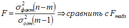
свободы. Fфакт > Fтеор — уравнение
регрессии адекватно.

n — число наблюдений
(уровней ряда), m — число параметров
уравнения (модели) регрессии.

Проверка
адекватности уравнения регрессии (
качества модели в целом) осуществляется
с помощью средней ошибки аппроксимации,
величина которой не должна превышать
10-12% (рекомендовано).

Соседние файлы в предмете [НЕСОРТИРОВАННОЕ]

Источник

Относительная ошибка аппроксимации это

Formal definition[edit]

Generalizations[edit]

Examples[edit]

Instruments[edit]

See also[edit]

References[edit]

External links[edit]

Formal definition[edit]

Generalizations[edit]

Examples[edit]

Instruments[edit]

See also[edit]

References[edit]

External links[edit]

Ошибки аппроксимации и ее определение.

Аналитический способ выравнивания временного ряда и используемые при этом функции.

А вот еще интересные материалы: