Computational Statistics with R
Hrishikesh D. Vinod, in Handbook of Statistics, 2014
6.3 Heteroscedastic and Autocorrelated Errors
If regression errors ϵ have nonconstant variances they are said to have heteroscedasticity. Sometimes a researcher may not want to correct this problem by using generalized least squares which changes the model. Then, all one can do is to test whether the presence of this problem makes regression coefficients statistically insignificant.
The usual variance–covariance matrix of regression coefficients used for testing the hypothesis that any component of β equals zero is given by cov(b)=s2(X′X)−1, where s2 is the residual variance. Prof. Hal White, an econometrician, and others have proposed to replace it by
(20)vcovHC(b)=s2(X′X)−1X′ΩX(X′X)−1,
where Ω is some known function representing the assumed pattern of changing variances. This is easily implemented in R by using the “vcovHC” function in the R package “sandwich” by Zeileis (2004), who also provides examples.
The three matrices in Eq. (20) have two outside matrices identical. Zeileis (2004) calls them “bread,” “meat,” and “bread” matrices. Statisticians working in robust estimators call them a Huber sandwich. Similar matrices arise in several estimation problems, including when regression errors have autocorrelation. Heteroskedasticity and autocorrelation consistent (HAC) estimation of variance–covariance matrix is given by his R function “vcovHAC” with similar syntax. If one wants to go beyond testing, Vinod (2010) provides new general approaches and R software tools to simultaneously correct for both of these problems, available at: http://www.fordham.edu/economics/vinod/autohetero.txt. This completes our discussion of matrix algebra R software tools used in the context of the regression model.
Read full chapter
URL:
https://www.sciencedirect.com/science/article/pii/B9780444634313000048
Scenario Analysis and Expected Credit Losses
Tiziano Bellini, in IFRS 9 and CECL Credit Risk Modelling and Validation, 2019
6.1 Introduction
IFRS 9 specifically requires projections under alternative scenarios and the adoption of a weighting scheme to compute ECL. FASB (2016) is not prescriptive in this regard. Nevertheless, no restrictions are imposed on this topic. Consequently, one may consider a multi-scenario setting both for IFRS 9 and CECL. Nonetheless, a reversion towards long-term mean loss rate is central under FASB (2016). Therefore two key issues need to be addressed in such a setting. On the one hand, one needs to specify a suitable time horizon for the reversion. On the other hand, a long-term loss rate needs to be estimated. Time series analysis plays a key role to address these issues. Based on this, structural models are often challenged by econometric methods to explain macroeconomic fluctuations. Flexibility and statistical reliability are the major advantages of vector auto-regression (VAR) and vector error-correction (VEC) models.
Three main goals inspire this chapter. Firstly, one needs to become familiar with the most common econometric tools to fit macroeconomic time series and make scenario projections. Secondly, we aim to bring together all credit risk components studied throughout the entire book to estimate ECL. The third goal is to create a framework to validate the overall ECL estimate. Indeed, risk component silos validation does not necessarily ensure a consistent ECL outcome.
Figure 6.1 summarizes how these three areas are investigated throughout the chapter.

Figure 6.1. Chapter’s workflow diagram.
- •
-
Scenario analysis. Section 6.2 introduces multivariate time series analysis. Details on how to perform VAR and VEC are provided. Since scenario analysis is at the very heart of the entire ECL computation, MVs analysis and impulse response analysis are studied. Some hints on global vector auto-regression (GVAR) modelling are also provided.
- •
-
ECL computation in practice. Credit risk models investigated throughout the book, together with scenarios above-detailed, are the key ingredients for computing ECL, as summarized in Section 6.3. In more detail, a practical guide on how to perform ECL computation is scrutinized by considering both IFRS 9 and CECL. Finally, the focus is on the staging allocation process prescribed by IASB (2014).
- •
-
ECL validation. In Section 6.4 the focus is on an overall ECL validation. Indeed, a silos risk parameter validation does not necessarily ensure a consistent ECL output. Two main perspectives are considered. On the one hand, historical credit losses are studied as a paradigm for ECL validation. On the other hand, a credit portfolio modelling perspective is followed to validate ECL results.
Examples and case studies are examined by means of R software throughout the chapter.
Read full chapter
URL:
https://www.sciencedirect.com/science/article/pii/B9780128149409000141
Regression Models
Robert Kissell, Jim Poserina, in Optimal Sports Math, Statistics, and Fantasy, 2017
Probability Home Team Wins
The probability that the actual outcome Y-variable will be less than or equal to a value S can be computed from the estimated Y-variable and regression error as follows:
Prob(Y≤S)=NormCdf(S,Yˆ,σy)
Here, NormCdf(S,Yˆ,σy) represents the cumulative normal distribution with mean=Yˆ and standard deviation=σy, and is the probability corresponding to a value less than or equal to S (see chapter: Advanced Math and Statistics, for detailed description of the calculation).
Subsequently, the probability that the home team will win a game if the expected outcome is Yˆ and the regression standard error is σy is calculated as follows:
Prob(HomeTeamWins)=1−NormCdf(0,Yˆ,σy)
This equation denotes the probability that the home team victory margin will be greater than zero and thus the home team wins the game.
Read full chapter
URL:
https://www.sciencedirect.com/science/article/pii/B9780128051634000025
Soccer—MLS
Robert Kissell, Jim Poserina, in Optimal Sports Math, Statistics, and Fantasy, 2017
9.9 Conclusion
In this chapter we applied six different sports model approaches to Major League Soccer results for the 2015 season. The models were used to predict winning team, estimated home team victory margin, and probability of winning. As with shootouts during regular-season NHL games, when predicting outcomes some consideration must be made for the large percentage of MLS matches, roughly one in five, that will end in a draw. All of the models had adjusted winning percentages in the neighborhood of 65%, with the team statistics model performing the best at 66.1%, despite the highest regression error and lowest regression R2 value of the six models. The logit spreads and logit points models had the next-best winning percentage, lowest regression error, and highest regression R2 values, followed by the other two probability models, logistic probability and team ratings.
We found that in all cases, these models performed better than the Vegas line using in-sample data and five of six of the models performed better than the Vegas line using out-sample data. The Logit Spread and Logit Points models had the highest goodness of fit (each with R2=65.5%) and the lowest regression (each with seY=1.57). These models performed better than the data driven models, but the Team Statistics model had the highest winning percentage at 66.1%. In all cases, our modeling approaches proved to be a valuable predictor of future game results including predicting winning team, winning spread, and probability of winning.
Read full chapter
URL:
https://www.sciencedirect.com/science/article/pii/B9780128051634000098
Simple linear regression
Stephen C. Loftus, in Basic Statistics with R, 2022
19.9.4 Assumption 4: homoskedasticity
The assumption that the variance of the errors is constant—referred to as homoskedasticity—is violated more often than one might think. In many real datasets, as the values of the response get larger the variability in the response also increases. Checking this error variance, unsurprisingly, involves our residuals as they are our proxies for the regression errors. As we did for checking linearity, to check homoskedasticity we plot our residuals versus the fitted values. As with linearity, if the errors are homoskedastic the residuals plotted against the fitted values will show a random scatter pattern. If we see a pattern, specifically a “fan pattern” similar to what is seen in Fig. 19.8, the errors are heteroskedastic and the assumption is violated.

Figure 19.8. A simulated dataset with the plot of predictor versus response and the residual plot showing heteroskedastic errors.
As with linearity, the residuals more clearly show the violation of the assumption than a plot of the raw data. In the Old Faithful regression, looking at Fig. 19.6 shows no fan pattern and thus the errors are homoskedastic. If the errors are heteroskedastic, in several cases a transformation of the response—similar to the linearity instance—will make the errors homoskedastic, thus satisfying the assumption.
Read full chapter
URL:
https://www.sciencedirect.com/science/article/pii/B9780128207888000328
Linear Models, Problems
John Fox, in Encyclopedia of Social Measurement, 2005
Measurement Error in the Explanatory Variables
Consider the following regression model:
yi=β1ξi+β2xi2+εi,
where the “latent” explanatory variable ξ is not directly observed (hence the Greek letter); x2 is directly observed and measured without error; and the regression error ɛ behaves according to the usual assumptions—in particular, E(ɛi) = 0, and the errors are uncorrelated with each other and with the explanatory variables. To simplify the exposition, but without loss of generality, suppose that all of the variables, y, ξ, and x2 (along with ɛ), have means of 0, eliminating the regression constant from the model. Imagine that we have a fallible observable indicator x1 of ξ,
xi1=ξi+δi,
where δ is the measurement-error component of x1. Suppose further that the measurement errors are “well behaved”: E(δ) = 0; E(ξδ) = 0 (the measurement errors and “true scores” are uncorrelated); E(x2δ) = 0 (the measurement errors in x1 are uncorrelated with the other explanatory variable); and E(ɛδ) = 0 (the measurement and regression errors are uncorrelated).
Under these circumstances, it is not hard to show that
(3)β1=σy1σ22−σ12σy2σ12σ22−σ122−σδ2σ22,β2=σy2σ12−σ12σy1σ12σ22−σ122−β1σ12σδ2σ12σ22−σ122
but that the population analogues of the least-squares coefficients (i.e., the quantities that the least-squares coefficients estimate) are
(4)β1′=σy1σ22−σ12σy2σ12σ22−σ122,β2′=σy2σ12−σ12σy1σ12σ22−σ122.
In these equations, the σ values are variances and covariances: for example, σy1 is the covariance of y and x1, σ12 is the variance of x1, and σδ2 is the measurement-error variance (which supposedly is nonzero). Comparing Eqs. (3) and (4) reveals that the least-squares coefficients are biased as estimators of β1 and β2: because the denominator of β1 in Eq. (3) must be positive, and −σδ2σ22 is necessarily negative, the least-squares estimand β′1 is “attenuated” toward zero.
The bias in β′2 has a different (and more interesting) characterization: Write β′2 = β2 + bias, where
bias=β1σ12σδ2σ12σ22−σ122.
The bias can be in either direction, but as the measurement-error variance σδ2 grows, the least-squares estimand β′2 is driven toward σy2/σ22, which is the population analogue of the least-squares coefficient for the regression of y on x2 alone. That is, a large measurement-error component in x1 makes it a weak statistical control, in effect removing it from the regression equation. Of course, when there are several explanatory variables, all subject to measurement error, the effects are more complex.
What can be done about measurement error in the predictors? Under certain circumstances—for example, when there are multiple indicators of latent explanatory variables—it is possible to derive unbiased estimators that take account of the measurement errors.
Read full chapter
URL:
https://www.sciencedirect.com/science/article/pii/B0123693985001651
Integrated modeling of the cobalt removal process
Chunhua Yang, Bei Sun, in Modeling, Optimization, and Control of Zinc Hydrometallurgical Purification Process, 2021
6.3.2 Working condition classification
In the CSS modeling framework, parameters of the FPM and the machine learning model under each working condition are different. To automatically classify the working condition, the deep features of ACP are first extracted. Then, the comprehensive state space is divided into subspaces using deep features. Each of the subspaces corresponds to a working condition.
6.3.2.1 Deep feature extraction
In order to decrease the computation load, the high-dimensional raw data have to be mapped into low-dimensional latent variables, which can be regarded as features of raw data. The mapping can be achieved using deep feature extraction (DFE), which can recognize the patterns of raw data. The advantage of DFE lies in its ability to learn very complex nonlinear functions. This is achieved using multiple levels of representation [12][13][14].
Stacked auto-encoder (SAE) is a typical unsupervised multilevel deep learning network [15]. In SAE, multiple auto-encoders are stacked to form a multilevel structure. In each auto-encoder, there exist one input layer, one output layer, and one hidden layer (Fig. 6.10). It first encodes the inputs to latent variables, and then the latent variables are used to reconstruct the inputs in the output layer. For the ith auto-encoder,

Figure 6.10. Deep feature extraction, regression, and subspace division.
(6.43)Yi=H(WiXi+bi),
(6.44)Yˆi=H′(Wi′Yi+bi′),
where Xi∈Rni is the input of an auto-encoder, Yi∈Rmi is the latent variables to be extracted, Yˆi∈Rni is the reconstructed outputs, H(⋅) and H′(⋅) are activation functions, e.g., sigmoid function, and Wi∈Rmi×ni, Wi′∈Rni×mi, bi∈Rmi, and bi′∈Rni are weighting matrices and bias vectors, which are the design parameters obtained by minimizing the reconstruction error on a training set with M samples:
(6.45)ℓSAE(Wi,Wi′,bi,bi′)=∑j=1M‖Xi(j)−Yˆi(j)‖2.
The extracted latent variables can be regarded as features of the inputs, which are then used as inputs of a subsequent auto-encoder. The training of SAE includes a pretraining and a fine-tuning stage. In the pretraining stage, the auto-encoders are trained layer by layer. After the pretraining of each auto-encoder, the latent variables of the last auto-encoder are outputted as the deep features z=YL. Then, the regression function U(z) is pretrained by minimizing the regression error:
(6.46)ℓRegression(α1,⋯,αN)=∑j=1M‖xOdeviation(j)−U(z(j))‖2,
where xOdeviation(j) and zi(j) are the FPM deviation and the deep features of the jth training sample, and U(⋅) is a regression function of the deep feature set z. After pretraining, [α1,⋯,αN] and [Wi,Wi′,bi,bi′] are used as initial guess to exploit the optimal weights by minimizing the overall regression error.
6.3.2.2 Deep feature space partitioning
The extracted deep features are then used to classify working conditions via dividing the comprehensive state space. In this study, the division of comprehensive state space is achieved in a sequential manner. The deep feature space is first divided. Then, the division of deep feature space is mapped back to the division of the comprehensive state space. In this section, the division of deep feature space is introduced, which involves a rough division and a fine division. In the rough division, a k-dimensional tree (KD-Tree) is applied to first divide the space into different partitions [16][17]. In the fine division, the result of rough division is fed as initial guess of an LR classifier to fine-tune the classification [18].
Rough division using a KD-Tree
KD-Tree is a variant of the binary tree. KD-Tree splits the deep feature space into two subspaces at each level iteratively until the deep feature space is divided into the desired number of subspaces (Fig. 6.11). The detailed steps of KD-Tree-based rough division include:
- Step 1:
-
Determine the desired numbers of partitions NP.
- Step 2:
-
Calculate the number of required features and the level of splits. If 2N−1<NP⩽2N, N⩾1, then N features and NS number of splits are required. We have
(6.47)NS=(2N−1−1)+(NP−2N−1)=NP−1.
- Step 3:
-
Normalize the deep features. Calculate the variances of the normalized features, and rank the features according to their variances. Let j=1.
- Step 4:
-
Calculate the median value of the jth feature. Consider the jth level, for partition S(j−1)q, where q=1 to 2(j−1), and generate a perpendicular splitting hyperplane which takes the median value on the axis of the jth feature. Then, the partition S(j−1)q is divided into two new subspaces Sj(2q−1),Sj(2q). These two new subspaces are ranked according to the variance of the (j+1)th feature.
- Step 5:
-
If j<N−1, then let j=j+1, and repeat Step 4 until j=N−1.
- Step 6:
-
If 2j<NP, then from q=1 to q=2j, divide the partition Sjq using the Nth feature until 2q+(2j−q)=NP.
After these steps, the original feature space S0 is partitioned into {SN1,SN2,⋯,SN(2q),Sj(q+1),⋯,Sj(2j)} (denoted as {S(1),S(2),⋯,S(NP)} hereafter).

Figure 6.11. Rough division using a KD-Tree.
Remark 1
In the rough division, the variance of deep features is selected as a division criterion. For each feature, larger feature variance corresponds to a wider distribution of feature values and therefore has a higher division efficiency [19].
Fine division based on LR
The KD-Tree approach roughly divides the deep feature space into different partitions, which can be used as an initial guess for the fine division. The fine division is achieved using LR classifier. It estimates and discriminates among the probabilities that the current process belongs to different working conditions:
(6.48)P(y|z)=11+e−σ(z),
(6.49)σ(z)=β0+∑i=1Nβizi,
where P(y|z) is the probability that the current observation z belongs to the working condition with label y. If P(y|z)>0.5, i.e., σ(z)>0, then z is considered as belonging to working condition y; σ(z)=0 is the decision boundary; β=[β0,β1,⋯,βN] is the coefficient set to be identified for each working condition.
The steps of fine division include:
- Step 1:
-
Let r=1.
- Step 2:
-
For subspace S(r), identify the coefficient set β(r) by minimizing the label estimation error:
(6.50)ℓLR(r)(β(r))=∑j=1M[11+e−σ(r)(zj)−y(j)]2=∑j=1M[11+e−[β0(r)+∑i=1Nβi(r)zi(j)]−y(j)]2,
where y(j) is the label of the jth sample given by rough division. The subspace surrounded by surface σ(r)(z)=0 is the rth subspace of the entire feature space.
- Step 3:
-
If r<NP, r=r+1, repeat Step 2.
Remark 2
The partition of the deep feature space can be mapped back to the partition of the comprehensive state space. However, the borders of the subspaces are not time-invariant. In addition, new types of working conditions may emerge during the production process. If a sufficient amount of data samples associated with new working conditions is generated, the deep feature space division should be repeated to update the partition.
Read full chapter
URL:
https://www.sciencedirect.com/science/article/pii/B978012819592500017X
Football—NFL
Robert Kissell, Jim Poserina, in Optimal Sports Math, Statistics, and Fantasy, 2017
6.1 Game Scores Model
The game scores regression model predicts game outcomes based on the average number of points scored and allowed by each team.
The model has the following form:
Y=b0+b1·HPS+b2·HPA+b3·APS+b4·APA+ε
In this representation, the dependent variable Y denotes the home team’s margin of victory (or defeat). A positive value indicates the home team won by the stated number of points and a negative value indicates the home team lost by the stated number of points.
The variables of this model are:
-
Y=home team victory margin
-
HPS=home team average points scored per game
-
HPA=home team average points allowed per game
-
APS=away team average points scored per game
-
APA=away team average points allowed per game
-
b0,b1,b2,b3,b4=model parameters, represents the sensitivities to the corresponding model factor.
The model parameters, i.e., betas, are determined from a linear regression analysis as described in Chapter 2, Regression Models.
The probability that the home team will be victorious is computed from the Excel normal distribution function as follows:
p=1−NormDist(0,Y,SeY,True)
Winning probability can also be computed from a statistical package such as via MATLAB’s normal cumulative distribution function as follows:
p=1−normcdf(0,Y,SeY)
Here, Y and SeY are the expected victory margin and regression error term respectively, and zero indicates the reference point used for the calculation (i.e., the probability that the winning margin will be greater than zero). This notation can be written more generally as:
Regression Results
The best fit regression equation for predicting the home team victory margin based on average points scored and average points allowed is below. Victory margin is positive when the home team is favored and negative when the visiting team is favored.
This model equation is:
VictoryMargin=−1.28+0.867·HPS−0.823·HPA−0.609·APS+0.999·APA±11.72
The game scores model returned a relatively high R2 value of R2=33%. The t-stats were −3.47 and 4.20 for visiting teams’ points scored and points allowed, and 4.99 and −3.48 for home teams, and an F-value of 32.08. The regression error was 11.72.
The signs of the input variables are intuitive. The sign of the parameter is expected to be positive for home points scored (HPS) and away points allowed (APA). In both of these cases, the home team will score more points if these input values are higher. Similarly, the signs of the parameters for home points allowed (HPA) and away team points scored (APS) are expected to be negative. The home team is expected to win by fewer points or possibly lose if the HPA and/or APS increase in value.
Table 6.2 shows the results of the regression model and Fig. 6.4 shows a graph of actual victory margin (spreads) compared to estimated victory margin (spreads) from our model.
Table 6.2. Game Scores Model: 2015 NFL
| Statistic | Value | t-Stat |
|---|---|---|
| b0 | −8.519 | −0.8 |
| b1 (Home points scored) | 0.867 | 5.0 |
| b2 (Home points allowed) | −0.823 | −3.5 |
| b3 (Visitor points scored) | −0.609 | −3.5 |
| b4 (Visitor points allowed) | 0.999 | 4.2 |
| R2 | 32.88% | |
| F-value | 32.082 | |
| Standard Error | 11.724 |

Figure 6.4. Game Scores Model: 2015 NFL.
Performance
The game scores model correctly identified the winner in 190 of 267 games, a rate of 71.2%. When the model gave the favorite at least a 60% win probability, the favorite won 78.5% of the time, and that figure jumped to 84.2% when the model predicted one team or the other as having a probability of winning of 70% or higher. Above 85%, the model was wrong only 3 times out of 46: a three-point loss by Baltimore to Pittsburgh in Week 4 in which the model had the Ravens as a 6-to-1 favorite, a two-point loss by Kansas City to Chicago in Week 5 in which the Bears were projected to be a 15½-point underdog, and a 35–28 defeat of the New England Patriots in Week 13 at the hands of the Philadelphia Eagles, who made the most of their 10.5% probability of winning.
For the 2015 NFL postseason, the model correctly predicted the winner in 9 of 11 games, missing only the Bengals’ loss to the Steelers in the first AFC Wild Card Game and the Broncos’ upset of the Panthers in Super Bowl 50, in which it had considered Carolina an 8-to-5 favorite.
The Vegas model predicted the winner 170 times out of 267 games for a winning percentage of 63.7%. The game scores regression predicted the winner 190 times out of 267 games for a winning percentage of 71.2%. Thus the game scores regression outperformed the Vegas line and won 21 more games.
The game scores regression won 66.3% of simulated spread bets against the Vegas line over the course of the 2015 NFL season, a record of 171–87–9. If the Vegas line was the Patriots by 9, the model bet on the Patriots when it predicted they would win by more than 9 points, and against the Patriots when it predicted they would win by fewer than 9 points or lose outright.
In the 2015 NFL postseason, the model won 9 of 11 times against the Vegas line, including both conference championship games. The only missed projections were the division game between Arizona and Green Bay and the Super Bowl, in which Vegas had the Panthers as 5-point favorite whereas the model projected a 6.7-point win by Carolina.
Rankings
The top 10 in the game scores model’s rankings all made the playoffs, as well as 11 of the top 12. The one playoff team not in the top 12 was the Washington Redskins, who ranked No. 14. The highest-ranked nonplayoff team was the New York Jets (10–6), who finished behind the 12–4 New England Patriots in the AFC East and lost the tiebreaker with the Pittsburgh Steelers for the AFC’s second wild card slot. The NFC champion Panthers were the No. 1 ranked team while the Super Bowl champion Broncos came in at No. 6, between the Cincinnati Bengals and the Steelers.
Example
We compare a game scenario between the Dallas Cowboys (4–12) at home versus the Oakland Raiders (7–9).
The 2015 Cowboys scored 17.2 points per game while allowing 23.4. The Raiders scored 22.4 points per game while their defense gave up 24.9 points per game. Given those averages and our regression results, the game scores model favors the Raiders in this game by 1.59 points:
VictoryMargin=−8.52+0.867(17.2)−0.823(23.4)−0.609(22.4)+0.999(24.9)=−1.59
The negative victory margin in this case indicates that the visiting team (Raiders) is the favored team by 1.59.
The corresponding probability that the host Cowboys would win is 45% and is calculated as follows:
p=1−NormCDF(0,−1.59,11.72)=44.62%
Read full chapter
URL:
https://www.sciencedirect.com/science/article/pii/B9780128051634000062
MORE REGRESSION METHODS
Rand R. Wilcox, in Applying Contemporary Statistical Techniques, 2003
14.7 Detecting Interactions
This section illustrates the methods previously covered in this chapter in the context of detecting interactions. Consider some outcome variable, Y, and two predictors, X1 and X2. Roughly, the issue is whether knowing the value of X2 modifies the association between Y and X1. For example, for the reading study introduced in Section 13.1, there was interest in how a measure of orthographic ability (Y) is related to a measure of auditory analysis, X1. A third variable in this study was a measure of sound blending (X2). Does knowing the value of this third variable alter the association between Y and X1; and if it does, how? More generally, there is interest in knowing whether a particular factor affects the magnitude of some effect size. Such factors are called moderators (e.g., Judd, Kenny, & McClelland, 2001).
Graphically, an interaction, in the context of regression, can be roughly described as follows. Let x2 be any value of the second predictor variable, X2. For example, x2 could be the median of the X2 values, but any other value could be used in what follows. Now consider the outcome variable, Y, and the first predictor (X1), and imagine that we split the n pairs of points (Y1,X11), …, (Yn, Xn1) into two groups: those pairs for which the corresponding X2 value is less than x2 and those for which the reverse is true. No interaction means that the regression lines corresponding to these two groups are parallel. For example, if for the first group Y=X12+∈ and for the second Y=X12+6+∈,, these regression lines are parallel and there is no interaction. But if for the second group Y=X12+8X1+3+∈,, say, then the regression lines intersect (at X1 = −3/8) and we say that X2 modifies the association between Y and X1.
A very popular method for checking and modeling interaction is with
(14.10)Y=β0+β1X1+β2X2+β3X1X2+∈.
That is, use the product of the two predictors to model interaction and conclude that an interaction exists if H0: β3 =0 can be rejected. (Saunders, 1955, 1956, appears to be the first to suggest this approach to detecting interactions in regression; cf. Cronbach, 1987; Baron & Kenny, 1986.) This hypothesis can be tested using methods already covered. That is, for the observations (Y1, X11, X12),…, (Yn, Xn1, Xn2), set Xi3 = Xi1Xi2 and for the model Y = β0 + β1X1 + β2X2 + β3X3 + ε, test N0: β3 = 0. However, it currently seems that a collection of tools is needed to address the issue of interactions in an adequate manner.
To add perspective on the product term just described, suppose we fix (or condition on) X2. That is, we treat it as a constant. Then a little algebra shows that Equation (14.10) can be written as
Y=(β0+β2X2)+(β1+β3X2)X1+∈.
So the intercept term becomes (β0 + β2X2) and the slope for X1 changes as a linear function of X2. If β3 = 0, then
Y=(β0+β2X2)+β1X1+∈.
That is, knowing X2 alters the intercept term but not the slope. Said another way, if we split the data into two groups according to whether X2 is less than or greater than some constant x2, the corresponding regression lines will be parallel, consistent with the description given earlier.
There are various ways one might model interaction in a more general fashion. For example, one could replace Equation (14.10) with
(14.11)Y=β0+β1X1+β2X2+g(X1X2)+∈
for some function g of the product. Equation (14.10) corresponds to the special case g(X1X2) = β3X1X2. A simple method for examining whether some function of the product might be useful is to create a partial residual plot as described in Section 14.2.5. This assumes, of course, that Y has a linear association with X1 and X2, and for the reading data, for example, we have already seen that this assumption seems dubious.
Before continuing, an exploratory tool is described that is useful when checking for a modifier variable; the method is based on a slight extension of the running-interval smoother. The basic idea is to plot the strength of the association between Y and X1 as a function of X2. Consider the ith observed value for X2, Xi2. Briefly, identify all of the Xj2 values that are close to Xi2 in the manner outlined in Section 14.2. Then for the corresponding pairs of points, (X1j, Yj), compute some correlation coefficient and label it θ^i.. Repeat this process for i = 1, …, n and then plot the pairs ((Xi2,θ^i).). The computations are performed by the S-PLUS function runcor described in Section 14.7.1 (cf. Doksum, Blyth, Bradlow, Meng, & Zhao, 1994).
EXAMPLE.
Some of the strategies that might be used to detect modifier variables are illustrated with data from a reading study previously mentioned. Again, we take as the outcome variable a measure of orhographic ability (Y), only this time the first predictor (X1) is a measure of sound blending and the issue is whether a measure of phonological awareness (X2) modifies the association between Y and X1. First consider the model given by Equation (14.10), where X3 = X1X2. If we apply the conventional F-test to H0: β1 = β2 = β3 = 0, the significance level is .044, but the significance levels for the three individual slope parameters are .46, .67, and .92, respectively. Estimating prediction error as described in Section 14.6, among the models
Y=β0+β1X1+∈,Y=β0+β2X2+∈,Y=β0+β3X3+∈,Y=β0+β1X1+β2X2+∈,Y=β0+β1X1+β2X2+β3X3+∈,
the first has the lowest prediction error (using least squares regression and squared error). This suggests that the first predictor is important but the others are not. But before making any final decisions about the associations under study, it is important to see whether other methods paint a different picture.
To get some feel for the data, Figure 14.9 shows a smooth created by the S-PLUS function runm3d, described in Section 14.2.4, when using X1 and X2 to predict Y. Notice that the regression surface does not appear tobe well approximated by a plane. That is, assuming a linear association might provide an inadequate representation of the data, contrary to what is typically assumed when investigating interactions.

FIGURE 14.9. A smooth for two predictors used in a reading study.
Next we examine the association between X1 and Y, ignoring X2 for the moment. Typically it is assumed that this association is linear and so one goal is to get some sense of whether this assumption is reasonable for the problem at hand. Figure 14.10 shows a smooth of these two variables that suggests a nonlinear association. Using the S-PLUS function linchk (described in Section 14.4.3) to check for linearity, with the data split at X1 = 7, the .95 confidence interval for the difference between the slopes is (−1.5,0) with a significance level of .027. The estimated slopes, using Theil–Sen, are 0 (for X1 < 7) and .5. Checking for linearity with the method in Box 14.1, the test statistic reported by the S-PLUS function lintest is 7.76 and the .05 critical value is 4.27, again suggesting that the hypothesis of a linear association is false. One way to proceed from here is to incorporate a measure of association that is sensitive to monotonic relationships that are not necessarily linear. Two classic approaches are available, but the details are postponed until Chapter 15. (For an analysis of these data based on one of these approaches, see the example in Section 15.12.) It is instructive, however, to proceed under the assumption that problems with nonlinearity can ignored.

FIGURE 14.10. A smooth based on the first of the two predictors used in the reading example.
Next we plot the smooth relating the (percentage bend) correlation between Y and X1 as a function of X2. Figure 14.11 shows the results based on the S-PLUS function runcor (described in Section 14.7.1). The + indicates the location of the median of X2, and the quartiles are indicated by a |. Note that the smooth is fairly horizontal on the left but that there is some indication that it begins to increase around X2 = 12 or perhaps X2 = 15. To provide perspective, the S-PLUS function runmean2g is used to simultaneously plot a smooth between Y and X1 based on points corresponding to X2 ≤ 12 as well as for X2 > 12. That is, runmean2g creates a smooth when predicting Y based on X1 for two groups. The first group corresponds to X2 ≤ 12, and the second is simply X2 > 12. (To facilitate this part of the analysis, the S-PLUS function regi, described in Section 14.7.1, is provided.) Figure 14.12 shows the results. Notice that for the second group (with points indicated by a +), there is only one point with X1 < 4. This means that the left portion of the smooth for the second group might be relatively inaccurate, for reasons mentioned in Section 14.1. Focusing on the X values in Figure 14.12 that are greater than or equal to 4, the two smooths appear to be fairly parallel, which suggests that there is no interaction. Also, curvature between Y and X1 now seems to be minimal. Testing the hypothesis of equal slopes with the S-PLUS function reg2ci using the Theil–Sen estimator, the significance level is .47, so we fail to reject and it might seem that it is safe to conclude that there is no interaction. The estimates of the slopes are 0 and .33.

FIGURE 14.11. A smooth based on the reading data that shows the percentage bend correlation between Y and X1 as a function of X2.

FIGURE 14.12. A smooth, based on the reading data, between Y and X1. The solid line is based on points with X2 ≤ 12 and the dashed line is for X2 ≥ 12.
There are, however, several concerns. The first is that for convenience, Theil–Sen was used. Checking for outliers using the MGV method and comparing the MGV regression estimate of the slope to Theil–Sen suggests that the slopes for the two groups are even more similar than indicated: The estimated slope for the second group drops slightly to .29. This might seem to support the conclusion that there is no interaction, but the MGV estimator can have a much smaller standard error, which could result in rejecting the hypothesis of equal slopes. Another concern is that the data were split according to whether X2 ≤ 12. Is this the optimal split for detecting an interaction? Empirical results previously described suggest splitting the data in this manner, but perhaps a slightly different split would make a practical difference. A third concern, which is always an issue when failing to reject, is whether power is sufficiently high to accept the null hypothesis of equal slopes. Addressing this problem for the problem at hand is difficult at best. And finally, it is unclear whether the apparent curvilinear association between X1 and Y can be ignored. (In Section 15.12, we will see that using a measure of association that is sensitive to this curvilinearity makes a practical difference.)
EXAMPLE.
The same two predictors in the previous example are used again, but now the outcome variable of interest (Y) is a measure of word accuracy and we consider whether phonological awareness modifies the association between sound blending and Y. Here we merely split the data into two groups according to whether X2 is less than or equal to its median. Checks on the second group indicate that a single unusual X1 value is seriously affecting the estimated slope based on both the Theil–Sen estimator and least squares. By restricting the range in this second group so as to eliminate this seemingly aberrant point, the .95 confidence interval for the difference between the slopes, using Theil–Sen, is (0, 4) with a significance level of .057 when testing the hypothesis that the slopes are equal. That is, for this particular split of the data, we are unable to reject at the .05 level the hypothesis that the two groups have unequal slopes. But we come fairly close to rejecting and concluding that phonological awareness modifies the association between sound blending and word accuracy. Testing the hypothesis that in Equation (14.10), β3 = 0, the significance level is .14 using least squares and the conventional Student’s T-test.
14.7.1 S-PLUS Functions runcor, regi, and cori
The S-PLUS function
runcor(x,y,z,fr=1,corflag=F,corfun=pbcor,plotit=T,rhat=F)
plots the correlation between x and y as a function of the data stored in the argument z. Setting the argument corflag to T (for true) results in using Pearson’s correlation; otherwise the function uses the correlation specified by the argument corfun, which defaults to the percentage bend correlation. Setting the argument rhat to T, the function returns the values of the estimated correlations corresponding to each value stored in z. For example, if the first value in z is 6, then the first value returned in rhat is the correlation between x and y for points for which the corresponding z values are close to 6. As usual, fr is the span and plotit=F will suppress the plot.
The S-PLUS function
regi(x,y,z,pt=median(z),fr=.8,est=mom,regfun=tsreg,testit=F,…)
creates two smooths. The first is based on the x and y values for which the corresponding value for z is less than the value stored in the argument pt. By default, pt is taken to be the median of the z values. The other smooth is based on the x and y values for which the corresponding value for z is greater than pt. The smooth is created with the measure of location given by the argument est, which defaults to MOM. If testit=T is used, the slopes (and intercepts) of the two regression lines, based on the function regfun (which defaults to the Theil–Sen estimator), are compared. (This is done by splitting the data for you and calling the function reg2ci.)
The S-PLUS function
cori(x,y,z,pt=median(z),fr=.8,est=mom,regfun=pbcor,testit=F,…)
is like regi, except that setting testit to T causes the correlations to be compared rather than the regression slopes. By default, the percentage bend correlation is used, but the argument corfun can be used to specify some other measure of association. (For example, corfun=spear results in using Spearman’s correlation, a measure of association covered in Chapter 15.)
Read full chapter
URL:
https://www.sciencedirect.com/science/article/pii/B9780127515410500353
Volume 3
J. Ferré, in Comprehensive Chemometrics, 2009
3.02.2.6 Residuals
A residual is the difference between an observed value and the corresponding value estimated by the model. Regression residuals can be calculated for the y-variable and also for the x-variables in the factor-based regression models (Section 3.02.2.7.3). Together with the analysis of the leverage, the analysis of the residuals (or of some improved transformation of them) is the basis of most diagnostic procedures for detecting failures in the model assumptions (Section 3.02.3.1) and highlighting problematic data points (Section 3.02.3.3). Below, we first deal with the ordinary residuals, directly obtained from the fitted model, and comment on their properties. Next, we describe transformations of the ordinary residuals to improve their performance as a diagnostic tool. The transformation is done by dividing the residual by a standard deviation. The choice of the standard deviation gives different scaled residuals with specific diagnostic power. It should be noted that these transformed residuals have different names in the literature. Finally, we comment on the recursive residuals that are used for the detection of autocorrelation.
3.02.2.6.1 Ordinary y-residuals
Equation (5) can be expressed in terms of the estimated coefficients as
(16)yi=b0+b1xi,1+…+bjxi,j+ei
where the difference between the observed yi and its value predicted by the model
(17)ei=yi−yˆi
is called the y-residual (also raw residual or ordinary residual) for the ith point. For all the observations, the vector of residuals is given by
(18)e=y−yˆ
One of the uses of the residuals is to provide an estimate of the variance of the error term. This is given by
(19)s2=eTeI−K
If the model is correct, this residual variance (also called residual mean square or mean-squared error, MSE) is an unbiased estimate of the unknown variance of the error σ2 (proof in, e.g., Myers,5 p 462). However, s2 is a biased estimate of σ2 if the model is underspecified or bad outliers are included. The numerator SSE = eTe is called sum of squares (SS) of the residuals (SSE) (also residual sum of squares (RSS) or sum of squared errors) and the square root of s2, s, is known as the standard error of estimate, standard error of calibration (SEC),27 or standard error of the regression (se). A standard error is the standard deviation of the probability distribution of the estimator.
3.02.2.6.1(i) Difference between ordinary residual and random error
Examination of the residuals is at the base of most regression diagnostics. Among other uses, the residuals are used for checking the assumptions we made on the errors (Section 3.02.2.3), and hence it is important to note the difference between residuals and errors. The errors ɛ are unobservable random variables. The ith residual ei can be regarded as an estimate of ɛi calculated from the observed data. Despite this, it is not always acceptable to assume that the residuals behave as the unobservable errors would. The residuals, unlike the errors, are correlated, and the ith residual ei is not only a function of ɛi but also a linear combination of all the errors ɛi (this is obtained by combining Equations (6), (11), and (18): e = y − Hy = (I − H) y = (I − H) (Xβ + ɛ) = (I − H) ɛ) (see Cook,2 p 11):
(20)ei=ɛi−∑n=1Ihinɛn
where hij is the (i,n) element of H. As the number of points I gets larger than the number of coefficients in the model, hij,(i≠j) tends to zero and ei ≈ ɛi, and the analysis of the residual distribution informs about the distribution of errors. However, for low I,hin,(i≠n) are larger and the contribution of the sum will not be negligible. Under the assumptions that the errors ɛ are independent random variables with mean zero and variance σ2, the residuals e have also mean zero:
(21)E(e)=0
and the variance–covariance matrix (see Draper and Smith,3 p 151)
(22)var(e)=(I−H)σ2
Moreover, if the vector of regression errors ɛ is normally distributed ɛ ∼ N(0,Iσ2), then the vector of regression residuals satisfies e ∼ N(0,(I − H)σ2). Equation (22) shows that each residual has a different variance, which depends on the location of the point in the regression space through the leverage hii:
(23)var(ei)=(1−hii)σ2
Points with x-values close to the data center have a small hii and var(ei) is close to σ2; points with extreme x-values have hii approaching to 1 and var(ei) approaching to 0. This small variance means that the residual for that extreme point will be small, that is, the model is shifted toward the yi of that point irrespective of the value of yi. Because the points with a large hii tend to be fitted more closely, they play a larger role in determining the estimated coefficients than points with smaller hii. In addition, as their ordinary residuals ei will be small, the diagnostics based on these residuals will be unsuccessful for signaling these large leverage points in case they are outliers.
3.02.2.6.2 Standardized y-residuals
The standardized residual is obtained by dividing the residual by the standard error of the regression as follows:
(24)es,i=eis
In addition to standardized residual,4 this type of residual has been called normalized residual,7 scaled residual,15 and unit normal deviate residual.3 Draper and Smith3 (p 144) comment that these residuals might be used as a rough approach for checking the normality assumption ɛi ∼ N(0, σ2) (i.e., ɛi/σ2 ∼ N(0, 1)). If ei and s are good estimates of ɛi and σ, then one can expect that these residuals follow approximately a normal distribution with zero mean and variance equal to one, es,i ≈ N(0, 1) if I is large, and a t distribution with I − K degrees of freedom if I is small. Under these assumptions, approximately 95% of the es,i should be in the interval [−2, 2]. This has also been used to derive the rule that residuals |es,i|>2 or |es,i|>3 may indicate an outlier (see Montgomery and Runger,28 p 396). Draper and Smith also warn that as the residuals ei are not independent and have nonconstant variance (and hence es,i neither are), checking these residuals might be misleading if var(ei) are too different. They recommend dividing the residual by an estimate of its own standard deviation, Equation (23). Two different ways of estimating the σ2 for Equation (23) lead to the two types of residuals commented next.
3.02.2.6.3 Internally studentized y-residuals
The internally studentized residual is calculated as
(25)ri=eis1−hii
In addition to internally studentized residual,2,14 this type of residual has been also called studentized residual4 and standardized residual.1,7,9,13,21 These residuals have mean zero and, unlike the ordinary residuals, they have unit variance (proof in Cook,2 p 19). Note that the numerator and denominator of ri are not independent because the numerator ei is used for calculating the standard deviation of the residuals (s) in the denominator. If point i is an outlier with a large ei, it will inflate s, which in turn will corrupt (decrease) ri. In addition, ri does not follow a t-distribution as ri* (Equation (26)) does.14 These residuals serve for the identification of heteroscedasticity (Section 3.02.3.1.2).
3.02.2.6.4 Externally studentized y-residuals
The externally studentized residual is calculated as
(26)ri*=eis−i1−hii
In addition to externally studentized residual,2,5,14,15 this type of residual has also been called studentized residual,1,9,21,24 deleted studentized residual,29 jackknife residual,4,7,15 and R-student.1,5 The difference between the externally and the internally studentized residual is that s−i (not s) is used as an estimate of the standard deviation σ. s−i has been calculated from a model without the observation i (Section 3.02.3.4.1) and hence s−i is independent of the residual ei. If the assumption of normality of errors ɛ holds, these residuals follow a Student’s t-distribution with I − K − 1 degrees of freedom, which can be used to assess their significance.30 The ri* will be large for those points that have large ordinary residuals and/or high leverage. However, even with a large leverage, ri* can be small if y is consistent with the model and the rest of the data. Note that ri and ri* are related as (see Cook,2 p 20)
(27)ri*=ri(I−K−1I−K−ri2)1/2
Although on occasions ri and ri* will be very similar, the ri* statistic is more sensitive (i.e., becomes larger) than ri in the presence of a discordant data point. The main discrepancy between them will arise when s and s−i are considerably different. This will happen when the ith observation exerts a large influence on the model (an hii value close to unity), and has a relatively large residual. These residuals serve for the identification of outliers. These residuals ri* are also the standardized form of the prediction sum of squares (PRESS) residuals (Section 3.02.3.4.1).
3.02.2.6.5 Recursive y-residuals
The recursive residuals31,32 are computed from a sequence of regressions starting with K observations and adding one observation at each step. Each regression equation is used to compute the residual for the next observation to be added as
(28)eir=yi−xiTbi−11+xiT(Xi−1TXi−1)−1xi,i=K+1,…,I
where bi−1 are estimated coefficients obtained from the first i−1 points and Xi−1 contains the first i−1 rows of X. This sequence continues until the last residual has been computed. There will be (I−K) recursive residuals, and the residuals from the first K observations are zero. If ɛi ∼ N(0, σ2), the recursive residuals are also eri ∼ N(0, σ2)32 when the model is correct. Hence, exact tests for normality and outliers can be used. These residuals allow the identification of autocorrelation, the detection of outliers,33 and also checking the assumptions of normality and homoscedasticity.34 Kianifard and Swallow35 reviewed the development and application of recursive residuals in linear models.
Read full chapter
URL:
https://www.sciencedirect.com/science/article/pii/B9780444527011000764
Computational Statistics with R
Hrishikesh D. Vinod, in Handbook of Statistics, 2014
6.3 Heteroscedastic and Autocorrelated Errors
If regression errors ϵ have nonconstant variances they are said to have heteroscedasticity. Sometimes a researcher may not want to correct this problem by using generalized least squares which changes the model. Then, all one can do is to test whether the presence of this problem makes regression coefficients statistically insignificant.
The usual variance–covariance matrix of regression coefficients used for testing the hypothesis that any component of β equals zero is given by cov(b)=s2(X′X)−1, where s2 is the residual variance. Prof. Hal White, an econometrician, and others have proposed to replace it by
(20)vcovHC(b)=s2(X′X)−1X′ΩX(X′X)−1,
where Ω is some known function representing the assumed pattern of changing variances. This is easily implemented in R by using the “vcovHC” function in the R package “sandwich” by Zeileis (2004), who also provides examples.
The three matrices in Eq. (20) have two outside matrices identical. Zeileis (2004) calls them “bread,” “meat,” and “bread” matrices. Statisticians working in robust estimators call them a Huber sandwich. Similar matrices arise in several estimation problems, including when regression errors have autocorrelation. Heteroskedasticity and autocorrelation consistent (HAC) estimation of variance–covariance matrix is given by his R function “vcovHAC” with similar syntax. If one wants to go beyond testing, Vinod (2010) provides new general approaches and R software tools to simultaneously correct for both of these problems, available at: http://www.fordham.edu/economics/vinod/autohetero.txt. This completes our discussion of matrix algebra R software tools used in the context of the regression model.
Read full chapter
URL:
https://www.sciencedirect.com/science/article/pii/B9780444634313000048
Scenario Analysis and Expected Credit Losses
Tiziano Bellini, in IFRS 9 and CECL Credit Risk Modelling and Validation, 2019
6.1 Introduction
IFRS 9 specifically requires projections under alternative scenarios and the adoption of a weighting scheme to compute ECL. FASB (2016) is not prescriptive in this regard. Nevertheless, no restrictions are imposed on this topic. Consequently, one may consider a multi-scenario setting both for IFRS 9 and CECL. Nonetheless, a reversion towards long-term mean loss rate is central under FASB (2016). Therefore two key issues need to be addressed in such a setting. On the one hand, one needs to specify a suitable time horizon for the reversion. On the other hand, a long-term loss rate needs to be estimated. Time series analysis plays a key role to address these issues. Based on this, structural models are often challenged by econometric methods to explain macroeconomic fluctuations. Flexibility and statistical reliability are the major advantages of vector auto-regression (VAR) and vector error-correction (VEC) models.
Three main goals inspire this chapter. Firstly, one needs to become familiar with the most common econometric tools to fit macroeconomic time series and make scenario projections. Secondly, we aim to bring together all credit risk components studied throughout the entire book to estimate ECL. The third goal is to create a framework to validate the overall ECL estimate. Indeed, risk component silos validation does not necessarily ensure a consistent ECL outcome.
Figure 6.1 summarizes how these three areas are investigated throughout the chapter.
Figure 6.1. Chapter’s workflow diagram.
- •
-
Scenario analysis. Section 6.2 introduces multivariate time series analysis. Details on how to perform VAR and VEC are provided. Since scenario analysis is at the very heart of the entire ECL computation, MVs analysis and impulse response analysis are studied. Some hints on global vector auto-regression (GVAR) modelling are also provided.
- •
-
ECL computation in practice. Credit risk models investigated throughout the book, together with scenarios above-detailed, are the key ingredients for computing ECL, as summarized in Section 6.3. In more detail, a practical guide on how to perform ECL computation is scrutinized by considering both IFRS 9 and CECL. Finally, the focus is on the staging allocation process prescribed by IASB (2014).
- •
-
ECL validation. In Section 6.4 the focus is on an overall ECL validation. Indeed, a silos risk parameter validation does not necessarily ensure a consistent ECL output. Two main perspectives are considered. On the one hand, historical credit losses are studied as a paradigm for ECL validation. On the other hand, a credit portfolio modelling perspective is followed to validate ECL results.
Examples and case studies are examined by means of R software throughout the chapter.
Read full chapter
URL:
https://www.sciencedirect.com/science/article/pii/B9780128149409000141
Regression Models
Robert Kissell, Jim Poserina, in Optimal Sports Math, Statistics, and Fantasy, 2017
Probability Home Team Wins
The probability that the actual outcome Y-variable will be less than or equal to a value S can be computed from the estimated Y-variable and regression error as follows:
Prob(Y≤S)=NormCdf(S,Yˆ,σy)
Here, NormCdf(S,Yˆ,σy) represents the cumulative normal distribution with mean=Yˆ and standard deviation=σy, and is the probability corresponding to a value less than or equal to S (see chapter: Advanced Math and Statistics, for detailed description of the calculation).
Subsequently, the probability that the home team will win a game if the expected outcome is Yˆ and the regression standard error is σy is calculated as follows:
Prob(HomeTeamWins)=1−NormCdf(0,Yˆ,σy)
This equation denotes the probability that the home team victory margin will be greater than zero and thus the home team wins the game.
Read full chapter
URL:
https://www.sciencedirect.com/science/article/pii/B9780128051634000025
Soccer—MLS
Robert Kissell, Jim Poserina, in Optimal Sports Math, Statistics, and Fantasy, 2017
9.9 Conclusion
In this chapter we applied six different sports model approaches to Major League Soccer results for the 2015 season. The models were used to predict winning team, estimated home team victory margin, and probability of winning. As with shootouts during regular-season NHL games, when predicting outcomes some consideration must be made for the large percentage of MLS matches, roughly one in five, that will end in a draw. All of the models had adjusted winning percentages in the neighborhood of 65%, with the team statistics model performing the best at 66.1%, despite the highest regression error and lowest regression R2 value of the six models. The logit spreads and logit points models had the next-best winning percentage, lowest regression error, and highest regression R2 values, followed by the other two probability models, logistic probability and team ratings.
We found that in all cases, these models performed better than the Vegas line using in-sample data and five of six of the models performed better than the Vegas line using out-sample data. The Logit Spread and Logit Points models had the highest goodness of fit (each with R2=65.5%) and the lowest regression (each with seY=1.57). These models performed better than the data driven models, but the Team Statistics model had the highest winning percentage at 66.1%. In all cases, our modeling approaches proved to be a valuable predictor of future game results including predicting winning team, winning spread, and probability of winning.
Read full chapter
URL:
https://www.sciencedirect.com/science/article/pii/B9780128051634000098
Simple linear regression
Stephen C. Loftus, in Basic Statistics with R, 2022
19.9.4 Assumption 4: homoskedasticity
The assumption that the variance of the errors is constant—referred to as homoskedasticity—is violated more often than one might think. In many real datasets, as the values of the response get larger the variability in the response also increases. Checking this error variance, unsurprisingly, involves our residuals as they are our proxies for the regression errors. As we did for checking linearity, to check homoskedasticity we plot our residuals versus the fitted values. As with linearity, if the errors are homoskedastic the residuals plotted against the fitted values will show a random scatter pattern. If we see a pattern, specifically a “fan pattern” similar to what is seen in Fig. 19.8, the errors are heteroskedastic and the assumption is violated.
Figure 19.8. A simulated dataset with the plot of predictor versus response and the residual plot showing heteroskedastic errors.
As with linearity, the residuals more clearly show the violation of the assumption than a plot of the raw data. In the Old Faithful regression, looking at Fig. 19.6 shows no fan pattern and thus the errors are homoskedastic. If the errors are heteroskedastic, in several cases a transformation of the response—similar to the linearity instance—will make the errors homoskedastic, thus satisfying the assumption.
Read full chapter
URL:
https://www.sciencedirect.com/science/article/pii/B9780128207888000328
Linear Models, Problems
John Fox, in Encyclopedia of Social Measurement, 2005
Measurement Error in the Explanatory Variables
Consider the following regression model:
yi=β1ξi+β2xi2+εi,
where the “latent” explanatory variable ξ is not directly observed (hence the Greek letter); x2 is directly observed and measured without error; and the regression error ɛ behaves according to the usual assumptions—in particular, E(ɛi) = 0, and the errors are uncorrelated with each other and with the explanatory variables. To simplify the exposition, but without loss of generality, suppose that all of the variables, y, ξ, and x2 (along with ɛ), have means of 0, eliminating the regression constant from the model. Imagine that we have a fallible observable indicator x1 of ξ,
xi1=ξi+δi,
where δ is the measurement-error component of x1. Suppose further that the measurement errors are “well behaved”: E(δ) = 0; E(ξδ) = 0 (the measurement errors and “true scores” are uncorrelated); E(x2δ) = 0 (the measurement errors in x1 are uncorrelated with the other explanatory variable); and E(ɛδ) = 0 (the measurement and regression errors are uncorrelated).
Under these circumstances, it is not hard to show that
(3)β1=σy1σ22−σ12σy2σ12σ22−σ122−σδ2σ22,β2=σy2σ12−σ12σy1σ12σ22−σ122−β1σ12σδ2σ12σ22−σ122
but that the population analogues of the least-squares coefficients (i.e., the quantities that the least-squares coefficients estimate) are
(4)β1′=σy1σ22−σ12σy2σ12σ22−σ122,β2′=σy2σ12−σ12σy1σ12σ22−σ122.
In these equations, the σ values are variances and covariances: for example, σy1 is the covariance of y and x1, σ12 is the variance of x1, and σδ2 is the measurement-error variance (which supposedly is nonzero). Comparing Eqs. (3) and (4) reveals that the least-squares coefficients are biased as estimators of β1 and β2: because the denominator of β1 in Eq. (3) must be positive, and −σδ2σ22 is necessarily negative, the least-squares estimand β′1 is “attenuated” toward zero.
The bias in β′2 has a different (and more interesting) characterization: Write β′2 = β2 + bias, where
bias=β1σ12σδ2σ12σ22−σ122.
The bias can be in either direction, but as the measurement-error variance σδ2 grows, the least-squares estimand β′2 is driven toward σy2/σ22, which is the population analogue of the least-squares coefficient for the regression of y on x2 alone. That is, a large measurement-error component in x1 makes it a weak statistical control, in effect removing it from the regression equation. Of course, when there are several explanatory variables, all subject to measurement error, the effects are more complex.
What can be done about measurement error in the predictors? Under certain circumstances—for example, when there are multiple indicators of latent explanatory variables—it is possible to derive unbiased estimators that take account of the measurement errors.
Read full chapter
URL:
https://www.sciencedirect.com/science/article/pii/B0123693985001651
Integrated modeling of the cobalt removal process
Chunhua Yang, Bei Sun, in Modeling, Optimization, and Control of Zinc Hydrometallurgical Purification Process, 2021
6.3.2 Working condition classification
In the CSS modeling framework, parameters of the FPM and the machine learning model under each working condition are different. To automatically classify the working condition, the deep features of ACP are first extracted. Then, the comprehensive state space is divided into subspaces using deep features. Each of the subspaces corresponds to a working condition.
6.3.2.1 Deep feature extraction
In order to decrease the computation load, the high-dimensional raw data have to be mapped into low-dimensional latent variables, which can be regarded as features of raw data. The mapping can be achieved using deep feature extraction (DFE), which can recognize the patterns of raw data. The advantage of DFE lies in its ability to learn very complex nonlinear functions. This is achieved using multiple levels of representation [12][13][14].
Stacked auto-encoder (SAE) is a typical unsupervised multilevel deep learning network [15]. In SAE, multiple auto-encoders are stacked to form a multilevel structure. In each auto-encoder, there exist one input layer, one output layer, and one hidden layer (Fig. 6.10). It first encodes the inputs to latent variables, and then the latent variables are used to reconstruct the inputs in the output layer. For the ith auto-encoder,
Figure 6.10. Deep feature extraction, regression, and subspace division.
(6.43)Yi=H(WiXi+bi),
(6.44)Yˆi=H′(Wi′Yi+bi′),
where Xi∈Rni is the input of an auto-encoder, Yi∈Rmi is the latent variables to be extracted, Yˆi∈Rni is the reconstructed outputs, H(⋅) and H′(⋅) are activation functions, e.g., sigmoid function, and Wi∈Rmi×ni, Wi′∈Rni×mi, bi∈Rmi, and bi′∈Rni are weighting matrices and bias vectors, which are the design parameters obtained by minimizing the reconstruction error on a training set with M samples:
(6.45)ℓSAE(Wi,Wi′,bi,bi′)=∑j=1M‖Xi(j)−Yˆi(j)‖2.
The extracted latent variables can be regarded as features of the inputs, which are then used as inputs of a subsequent auto-encoder. The training of SAE includes a pretraining and a fine-tuning stage. In the pretraining stage, the auto-encoders are trained layer by layer. After the pretraining of each auto-encoder, the latent variables of the last auto-encoder are outputted as the deep features z=YL. Then, the regression function U(z) is pretrained by minimizing the regression error:
(6.46)ℓRegression(α1,⋯,αN)=∑j=1M‖xOdeviation(j)−U(z(j))‖2,
where xOdeviation(j) and zi(j) are the FPM deviation and the deep features of the jth training sample, and U(⋅) is a regression function of the deep feature set z. After pretraining, [α1,⋯,αN] and [Wi,Wi′,bi,bi′] are used as initial guess to exploit the optimal weights by minimizing the overall regression error.
6.3.2.2 Deep feature space partitioning
The extracted deep features are then used to classify working conditions via dividing the comprehensive state space. In this study, the division of comprehensive state space is achieved in a sequential manner. The deep feature space is first divided. Then, the division of deep feature space is mapped back to the division of the comprehensive state space. In this section, the division of deep feature space is introduced, which involves a rough division and a fine division. In the rough division, a k-dimensional tree (KD-Tree) is applied to first divide the space into different partitions [16][17]. In the fine division, the result of rough division is fed as initial guess of an LR classifier to fine-tune the classification [18].
Rough division using a KD-Tree
KD-Tree is a variant of the binary tree. KD-Tree splits the deep feature space into two subspaces at each level iteratively until the deep feature space is divided into the desired number of subspaces (Fig. 6.11). The detailed steps of KD-Tree-based rough division include:
- Step 1:
-
Determine the desired numbers of partitions NP.
- Step 2:
-
Calculate the number of required features and the level of splits. If 2N−1<NP⩽2N, N⩾1, then N features and NS number of splits are required. We have
(6.47)NS=(2N−1−1)+(NP−2N−1)=NP−1.
- Step 3:
-
Normalize the deep features. Calculate the variances of the normalized features, and rank the features according to their variances. Let j=1.
- Step 4:
-
Calculate the median value of the jth feature. Consider the jth level, for partition S(j−1)q, where q=1 to 2(j−1), and generate a perpendicular splitting hyperplane which takes the median value on the axis of the jth feature. Then, the partition S(j−1)q is divided into two new subspaces Sj(2q−1),Sj(2q). These two new subspaces are ranked according to the variance of the (j+1)th feature.
- Step 5:
-
If j<N−1, then let j=j+1, and repeat Step 4 until j=N−1.
- Step 6:
-
If 2j<NP, then from q=1 to q=2j, divide the partition Sjq using the Nth feature until 2q+(2j−q)=NP.
After these steps, the original feature space S0 is partitioned into {SN1,SN2,⋯,SN(2q),Sj(q+1),⋯,Sj(2j)} (denoted as {S(1),S(2),⋯,S(NP)} hereafter).
Figure 6.11. Rough division using a KD-Tree.
Remark 1
In the rough division, the variance of deep features is selected as a division criterion. For each feature, larger feature variance corresponds to a wider distribution of feature values and therefore has a higher division efficiency [19].
Fine division based on LR
The KD-Tree approach roughly divides the deep feature space into different partitions, which can be used as an initial guess for the fine division. The fine division is achieved using LR classifier. It estimates and discriminates among the probabilities that the current process belongs to different working conditions:
(6.48)P(y|z)=11+e−σ(z),
(6.49)σ(z)=β0+∑i=1Nβizi,
where P(y|z) is the probability that the current observation z belongs to the working condition with label y. If P(y|z)>0.5, i.e., σ(z)>0, then z is considered as belonging to working condition y; σ(z)=0 is the decision boundary; β=[β0,β1,⋯,βN] is the coefficient set to be identified for each working condition.
The steps of fine division include:
- Step 1:
-
Let r=1.
- Step 2:
-
For subspace S(r), identify the coefficient set β(r) by minimizing the label estimation error:
(6.50)ℓLR(r)(β(r))=∑j=1M[11+e−σ(r)(zj)−y(j)]2=∑j=1M[11+e−[β0(r)+∑i=1Nβi(r)zi(j)]−y(j)]2,
where y(j) is the label of the jth sample given by rough division. The subspace surrounded by surface σ(r)(z)=0 is the rth subspace of the entire feature space.
- Step 3:
-
If r<NP, r=r+1, repeat Step 2.
Remark 2
The partition of the deep feature space can be mapped back to the partition of the comprehensive state space. However, the borders of the subspaces are not time-invariant. In addition, new types of working conditions may emerge during the production process. If a sufficient amount of data samples associated with new working conditions is generated, the deep feature space division should be repeated to update the partition.
Read full chapter
URL:
https://www.sciencedirect.com/science/article/pii/B978012819592500017X
Football—NFL
Robert Kissell, Jim Poserina, in Optimal Sports Math, Statistics, and Fantasy, 2017
6.1 Game Scores Model
The game scores regression model predicts game outcomes based on the average number of points scored and allowed by each team.
The model has the following form:
Y=b0+b1·HPS+b2·HPA+b3·APS+b4·APA+ε
In this representation, the dependent variable Y denotes the home team’s margin of victory (or defeat). A positive value indicates the home team won by the stated number of points and a negative value indicates the home team lost by the stated number of points.
The variables of this model are:
-
Y=home team victory margin
-
HPS=home team average points scored per game
-
HPA=home team average points allowed per game
-
APS=away team average points scored per game
-
APA=away team average points allowed per game
-
b0,b1,b2,b3,b4=model parameters, represents the sensitivities to the corresponding model factor.
The model parameters, i.e., betas, are determined from a linear regression analysis as described in Chapter 2, Regression Models.
The probability that the home team will be victorious is computed from the Excel normal distribution function as follows:
p=1−NormDist(0,Y,SeY,True)
Winning probability can also be computed from a statistical package such as via MATLAB’s normal cumulative distribution function as follows:
p=1−normcdf(0,Y,SeY)
Here, Y and SeY are the expected victory margin and regression error term respectively, and zero indicates the reference point used for the calculation (i.e., the probability that the winning margin will be greater than zero). This notation can be written more generally as:
Regression Results
The best fit regression equation for predicting the home team victory margin based on average points scored and average points allowed is below. Victory margin is positive when the home team is favored and negative when the visiting team is favored.
This model equation is:
VictoryMargin=−1.28+0.867·HPS−0.823·HPA−0.609·APS+0.999·APA±11.72
The game scores model returned a relatively high R2 value of R2=33%. The t-stats were −3.47 and 4.20 for visiting teams’ points scored and points allowed, and 4.99 and −3.48 for home teams, and an F-value of 32.08. The regression error was 11.72.
The signs of the input variables are intuitive. The sign of the parameter is expected to be positive for home points scored (HPS) and away points allowed (APA). In both of these cases, the home team will score more points if these input values are higher. Similarly, the signs of the parameters for home points allowed (HPA) and away team points scored (APS) are expected to be negative. The home team is expected to win by fewer points or possibly lose if the HPA and/or APS increase in value.
Table 6.2 shows the results of the regression model and Fig. 6.4 shows a graph of actual victory margin (spreads) compared to estimated victory margin (spreads) from our model.
Table 6.2. Game Scores Model: 2015 NFL
| Statistic | Value | t-Stat |
|---|---|---|
| b0 | −8.519 | −0.8 |
| b1 (Home points scored) | 0.867 | 5.0 |
| b2 (Home points allowed) | −0.823 | −3.5 |
| b3 (Visitor points scored) | −0.609 | −3.5 |
| b4 (Visitor points allowed) | 0.999 | 4.2 |
| R2 | 32.88% | |
| F-value | 32.082 | |
| Standard Error | 11.724 |
Figure 6.4. Game Scores Model: 2015 NFL.
Performance
The game scores model correctly identified the winner in 190 of 267 games, a rate of 71.2%. When the model gave the favorite at least a 60% win probability, the favorite won 78.5% of the time, and that figure jumped to 84.2% when the model predicted one team or the other as having a probability of winning of 70% or higher. Above 85%, the model was wrong only 3 times out of 46: a three-point loss by Baltimore to Pittsburgh in Week 4 in which the model had the Ravens as a 6-to-1 favorite, a two-point loss by Kansas City to Chicago in Week 5 in which the Bears were projected to be a 15½-point underdog, and a 35–28 defeat of the New England Patriots in Week 13 at the hands of the Philadelphia Eagles, who made the most of their 10.5% probability of winning.
For the 2015 NFL postseason, the model correctly predicted the winner in 9 of 11 games, missing only the Bengals’ loss to the Steelers in the first AFC Wild Card Game and the Broncos’ upset of the Panthers in Super Bowl 50, in which it had considered Carolina an 8-to-5 favorite.
The Vegas model predicted the winner 170 times out of 267 games for a winning percentage of 63.7%. The game scores regression predicted the winner 190 times out of 267 games for a winning percentage of 71.2%. Thus the game scores regression outperformed the Vegas line and won 21 more games.
The game scores regression won 66.3% of simulated spread bets against the Vegas line over the course of the 2015 NFL season, a record of 171–87–9. If the Vegas line was the Patriots by 9, the model bet on the Patriots when it predicted they would win by more than 9 points, and against the Patriots when it predicted they would win by fewer than 9 points or lose outright.
In the 2015 NFL postseason, the model won 9 of 11 times against the Vegas line, including both conference championship games. The only missed projections were the division game between Arizona and Green Bay and the Super Bowl, in which Vegas had the Panthers as 5-point favorite whereas the model projected a 6.7-point win by Carolina.
Rankings
The top 10 in the game scores model’s rankings all made the playoffs, as well as 11 of the top 12. The one playoff team not in the top 12 was the Washington Redskins, who ranked No. 14. The highest-ranked nonplayoff team was the New York Jets (10–6), who finished behind the 12–4 New England Patriots in the AFC East and lost the tiebreaker with the Pittsburgh Steelers for the AFC’s second wild card slot. The NFC champion Panthers were the No. 1 ranked team while the Super Bowl champion Broncos came in at No. 6, between the Cincinnati Bengals and the Steelers.
Example
We compare a game scenario between the Dallas Cowboys (4–12) at home versus the Oakland Raiders (7–9).
The 2015 Cowboys scored 17.2 points per game while allowing 23.4. The Raiders scored 22.4 points per game while their defense gave up 24.9 points per game. Given those averages and our regression results, the game scores model favors the Raiders in this game by 1.59 points:
VictoryMargin=−8.52+0.867(17.2)−0.823(23.4)−0.609(22.4)+0.999(24.9)=−1.59
The negative victory margin in this case indicates that the visiting team (Raiders) is the favored team by 1.59.
The corresponding probability that the host Cowboys would win is 45% and is calculated as follows:
p=1−NormCDF(0,−1.59,11.72)=44.62%
Read full chapter
URL:
https://www.sciencedirect.com/science/article/pii/B9780128051634000062
MORE REGRESSION METHODS
Rand R. Wilcox, in Applying Contemporary Statistical Techniques, 2003
14.7 Detecting Interactions
This section illustrates the methods previously covered in this chapter in the context of detecting interactions. Consider some outcome variable, Y, and two predictors, X1 and X2. Roughly, the issue is whether knowing the value of X2 modifies the association between Y and X1. For example, for the reading study introduced in Section 13.1, there was interest in how a measure of orthographic ability (Y) is related to a measure of auditory analysis, X1. A third variable in this study was a measure of sound blending (X2). Does knowing the value of this third variable alter the association between Y and X1; and if it does, how? More generally, there is interest in knowing whether a particular factor affects the magnitude of some effect size. Such factors are called moderators (e.g., Judd, Kenny, & McClelland, 2001).
Graphically, an interaction, in the context of regression, can be roughly described as follows. Let x2 be any value of the second predictor variable, X2. For example, x2 could be the median of the X2 values, but any other value could be used in what follows. Now consider the outcome variable, Y, and the first predictor (X1), and imagine that we split the n pairs of points (Y1,X11), …, (Yn, Xn1) into two groups: those pairs for which the corresponding X2 value is less than x2 and those for which the reverse is true. No interaction means that the regression lines corresponding to these two groups are parallel. For example, if for the first group Y=X12+∈ and for the second Y=X12+6+∈,, these regression lines are parallel and there is no interaction. But if for the second group Y=X12+8X1+3+∈,, say, then the regression lines intersect (at X1 = −3/8) and we say that X2 modifies the association between Y and X1.
A very popular method for checking and modeling interaction is with
(14.10)Y=β0+β1X1+β2X2+β3X1X2+∈.
That is, use the product of the two predictors to model interaction and conclude that an interaction exists if H0: β3 =0 can be rejected. (Saunders, 1955, 1956, appears to be the first to suggest this approach to detecting interactions in regression; cf. Cronbach, 1987; Baron & Kenny, 1986.) This hypothesis can be tested using methods already covered. That is, for the observations (Y1, X11, X12),…, (Yn, Xn1, Xn2), set Xi3 = Xi1Xi2 and for the model Y = β0 + β1X1 + β2X2 + β3X3 + ε, test N0: β3 = 0. However, it currently seems that a collection of tools is needed to address the issue of interactions in an adequate manner.
To add perspective on the product term just described, suppose we fix (or condition on) X2. That is, we treat it as a constant. Then a little algebra shows that Equation (14.10) can be written as
Y=(β0+β2X2)+(β1+β3X2)X1+∈.
So the intercept term becomes (β0 + β2X2) and the slope for X1 changes as a linear function of X2. If β3 = 0, then
Y=(β0+β2X2)+β1X1+∈.
That is, knowing X2 alters the intercept term but not the slope. Said another way, if we split the data into two groups according to whether X2 is less than or greater than some constant x2, the corresponding regression lines will be parallel, consistent with the description given earlier.
There are various ways one might model interaction in a more general fashion. For example, one could replace Equation (14.10) with
(14.11)Y=β0+β1X1+β2X2+g(X1X2)+∈
for some function g of the product. Equation (14.10) corresponds to the special case g(X1X2) = β3X1X2. A simple method for examining whether some function of the product might be useful is to create a partial residual plot as described in Section 14.2.5. This assumes, of course, that Y has a linear association with X1 and X2, and for the reading data, for example, we have already seen that this assumption seems dubious.
Before continuing, an exploratory tool is described that is useful when checking for a modifier variable; the method is based on a slight extension of the running-interval smoother. The basic idea is to plot the strength of the association between Y and X1 as a function of X2. Consider the ith observed value for X2, Xi2. Briefly, identify all of the Xj2 values that are close to Xi2 in the manner outlined in Section 14.2. Then for the corresponding pairs of points, (X1j, Yj), compute some correlation coefficient and label it θ^i.. Repeat this process for i = 1, …, n and then plot the pairs ((Xi2,θ^i).). The computations are performed by the S-PLUS function runcor described in Section 14.7.1 (cf. Doksum, Blyth, Bradlow, Meng, & Zhao, 1994).
EXAMPLE.
Some of the strategies that might be used to detect modifier variables are illustrated with data from a reading study previously mentioned. Again, we take as the outcome variable a measure of orhographic ability (Y), only this time the first predictor (X1) is a measure of sound blending and the issue is whether a measure of phonological awareness (X2) modifies the association between Y and X1. First consider the model given by Equation (14.10), where X3 = X1X2. If we apply the conventional F-test to H0: β1 = β2 = β3 = 0, the significance level is .044, but the significance levels for the three individual slope parameters are .46, .67, and .92, respectively. Estimating prediction error as described in Section 14.6, among the models
Y=β0+β1X1+∈,Y=β0+β2X2+∈,Y=β0+β3X3+∈,Y=β0+β1X1+β2X2+∈,Y=β0+β1X1+β2X2+β3X3+∈,
the first has the lowest prediction error (using least squares regression and squared error). This suggests that the first predictor is important but the others are not. But before making any final decisions about the associations under study, it is important to see whether other methods paint a different picture.
To get some feel for the data, Figure 14.9 shows a smooth created by the S-PLUS function runm3d, described in Section 14.2.4, when using X1 and X2 to predict Y. Notice that the regression surface does not appear tobe well approximated by a plane. That is, assuming a linear association might provide an inadequate representation of the data, contrary to what is typically assumed when investigating interactions.
FIGURE 14.9. A smooth for two predictors used in a reading study.
Next we examine the association between X1 and Y, ignoring X2 for the moment. Typically it is assumed that this association is linear and so one goal is to get some sense of whether this assumption is reasonable for the problem at hand. Figure 14.10 shows a smooth of these two variables that suggests a nonlinear association. Using the S-PLUS function linchk (described in Section 14.4.3) to check for linearity, with the data split at X1 = 7, the .95 confidence interval for the difference between the slopes is (−1.5,0) with a significance level of .027. The estimated slopes, using Theil–Sen, are 0 (for X1 < 7) and .5. Checking for linearity with the method in Box 14.1, the test statistic reported by the S-PLUS function lintest is 7.76 and the .05 critical value is 4.27, again suggesting that the hypothesis of a linear association is false. One way to proceed from here is to incorporate a measure of association that is sensitive to monotonic relationships that are not necessarily linear. Two classic approaches are available, but the details are postponed until Chapter 15. (For an analysis of these data based on one of these approaches, see the example in Section 15.12.) It is instructive, however, to proceed under the assumption that problems with nonlinearity can ignored.
FIGURE 14.10. A smooth based on the first of the two predictors used in the reading example.
Next we plot the smooth relating the (percentage bend) correlation between Y and X1 as a function of X2. Figure 14.11 shows the results based on the S-PLUS function runcor (described in Section 14.7.1). The + indicates the location of the median of X2, and the quartiles are indicated by a |. Note that the smooth is fairly horizontal on the left but that there is some indication that it begins to increase around X2 = 12 or perhaps X2 = 15. To provide perspective, the S-PLUS function runmean2g is used to simultaneously plot a smooth between Y and X1 based on points corresponding to X2 ≤ 12 as well as for X2 > 12. That is, runmean2g creates a smooth when predicting Y based on X1 for two groups. The first group corresponds to X2 ≤ 12, and the second is simply X2 > 12. (To facilitate this part of the analysis, the S-PLUS function regi, described in Section 14.7.1, is provided.) Figure 14.12 shows the results. Notice that for the second group (with points indicated by a +), there is only one point with X1 < 4. This means that the left portion of the smooth for the second group might be relatively inaccurate, for reasons mentioned in Section 14.1. Focusing on the X values in Figure 14.12 that are greater than or equal to 4, the two smooths appear to be fairly parallel, which suggests that there is no interaction. Also, curvature between Y and X1 now seems to be minimal. Testing the hypothesis of equal slopes with the S-PLUS function reg2ci using the Theil–Sen estimator, the significance level is .47, so we fail to reject and it might seem that it is safe to conclude that there is no interaction. The estimates of the slopes are 0 and .33.
FIGURE 14.11. A smooth based on the reading data that shows the percentage bend correlation between Y and X1 as a function of X2.
FIGURE 14.12. A smooth, based on the reading data, between Y and X1. The solid line is based on points with X2 ≤ 12 and the dashed line is for X2 ≥ 12.
There are, however, several concerns. The first is that for convenience, Theil–Sen was used. Checking for outliers using the MGV method and comparing the MGV regression estimate of the slope to Theil–Sen suggests that the slopes for the two groups are even more similar than indicated: The estimated slope for the second group drops slightly to .29. This might seem to support the conclusion that there is no interaction, but the MGV estimator can have a much smaller standard error, which could result in rejecting the hypothesis of equal slopes. Another concern is that the data were split according to whether X2 ≤ 12. Is this the optimal split for detecting an interaction? Empirical results previously described suggest splitting the data in this manner, but perhaps a slightly different split would make a practical difference. A third concern, which is always an issue when failing to reject, is whether power is sufficiently high to accept the null hypothesis of equal slopes. Addressing this problem for the problem at hand is difficult at best. And finally, it is unclear whether the apparent curvilinear association between X1 and Y can be ignored. (In Section 15.12, we will see that using a measure of association that is sensitive to this curvilinearity makes a practical difference.)
EXAMPLE.
The same two predictors in the previous example are used again, but now the outcome variable of interest (Y) is a measure of word accuracy and we consider whether phonological awareness modifies the association between sound blending and Y. Here we merely split the data into two groups according to whether X2 is less than or equal to its median. Checks on the second group indicate that a single unusual X1 value is seriously affecting the estimated slope based on both the Theil–Sen estimator and least squares. By restricting the range in this second group so as to eliminate this seemingly aberrant point, the .95 confidence interval for the difference between the slopes, using Theil–Sen, is (0, 4) with a significance level of .057 when testing the hypothesis that the slopes are equal. That is, for this particular split of the data, we are unable to reject at the .05 level the hypothesis that the two groups have unequal slopes. But we come fairly close to rejecting and concluding that phonological awareness modifies the association between sound blending and word accuracy. Testing the hypothesis that in Equation (14.10), β3 = 0, the significance level is .14 using least squares and the conventional Student’s T-test.
14.7.1 S-PLUS Functions runcor, regi, and cori
The S-PLUS function
runcor(x,y,z,fr=1,corflag=F,corfun=pbcor,plotit=T,rhat=F)
plots the correlation between x and y as a function of the data stored in the argument z. Setting the argument corflag to T (for true) results in using Pearson’s correlation; otherwise the function uses the correlation specified by the argument corfun, which defaults to the percentage bend correlation. Setting the argument rhat to T, the function returns the values of the estimated correlations corresponding to each value stored in z. For example, if the first value in z is 6, then the first value returned in rhat is the correlation between x and y for points for which the corresponding z values are close to 6. As usual, fr is the span and plotit=F will suppress the plot.
The S-PLUS function
regi(x,y,z,pt=median(z),fr=.8,est=mom,regfun=tsreg,testit=F,…)
creates two smooths. The first is based on the x and y values for which the corresponding value for z is less than the value stored in the argument pt. By default, pt is taken to be the median of the z values. The other smooth is based on the x and y values for which the corresponding value for z is greater than pt. The smooth is created with the measure of location given by the argument est, which defaults to MOM. If testit=T is used, the slopes (and intercepts) of the two regression lines, based on the function regfun (which defaults to the Theil–Sen estimator), are compared. (This is done by splitting the data for you and calling the function reg2ci.)
The S-PLUS function
cori(x,y,z,pt=median(z),fr=.8,est=mom,regfun=pbcor,testit=F,…)
is like regi, except that setting testit to T causes the correlations to be compared rather than the regression slopes. By default, the percentage bend correlation is used, but the argument corfun can be used to specify some other measure of association. (For example, corfun=spear results in using Spearman’s correlation, a measure of association covered in Chapter 15.)
Read full chapter
URL:
https://www.sciencedirect.com/science/article/pii/B9780127515410500353
Volume 3
J. Ferré, in Comprehensive Chemometrics, 2009
3.02.2.6 Residuals
A residual is the difference between an observed value and the corresponding value estimated by the model. Regression residuals can be calculated for the y-variable and also for the x-variables in the factor-based regression models (Section 3.02.2.7.3). Together with the analysis of the leverage, the analysis of the residuals (or of some improved transformation of them) is the basis of most diagnostic procedures for detecting failures in the model assumptions (Section 3.02.3.1) and highlighting problematic data points (Section 3.02.3.3). Below, we first deal with the ordinary residuals, directly obtained from the fitted model, and comment on their properties. Next, we describe transformations of the ordinary residuals to improve their performance as a diagnostic tool. The transformation is done by dividing the residual by a standard deviation. The choice of the standard deviation gives different scaled residuals with specific diagnostic power. It should be noted that these transformed residuals have different names in the literature. Finally, we comment on the recursive residuals that are used for the detection of autocorrelation.
3.02.2.6.1 Ordinary y-residuals
Equation (5) can be expressed in terms of the estimated coefficients as
(16)yi=b0+b1xi,1+…+bjxi,j+ei
where the difference between the observed yi and its value predicted by the model
(17)ei=yi−yˆi
is called the y-residual (also raw residual or ordinary residual) for the ith point. For all the observations, the vector of residuals is given by
(18)e=y−yˆ
One of the uses of the residuals is to provide an estimate of the variance of the error term. This is given by
(19)s2=eTeI−K
If the model is correct, this residual variance (also called residual mean square or mean-squared error, MSE) is an unbiased estimate of the unknown variance of the error σ2 (proof in, e.g., Myers,5 p 462). However, s2 is a biased estimate of σ2 if the model is underspecified or bad outliers are included. The numerator SSE = eTe is called sum of squares (SS) of the residuals (SSE) (also residual sum of squares (RSS) or sum of squared errors) and the square root of s2, s, is known as the standard error of estimate, standard error of calibration (SEC),27 or standard error of the regression (se). A standard error is the standard deviation of the probability distribution of the estimator.
3.02.2.6.1(i) Difference between ordinary residual and random error
Examination of the residuals is at the base of most regression diagnostics. Among other uses, the residuals are used for checking the assumptions we made on the errors (Section 3.02.2.3), and hence it is important to note the difference between residuals and errors. The errors ɛ are unobservable random variables. The ith residual ei can be regarded as an estimate of ɛi calculated from the observed data. Despite this, it is not always acceptable to assume that the residuals behave as the unobservable errors would. The residuals, unlike the errors, are correlated, and the ith residual ei is not only a function of ɛi but also a linear combination of all the errors ɛi (this is obtained by combining Equations (6), (11), and (18): e = y − Hy = (I − H) y = (I − H) (Xβ + ɛ) = (I − H) ɛ) (see Cook,2 p 11):
(20)ei=ɛi−∑n=1Ihinɛn
where hij is the (i,n) element of H. As the number of points I gets larger than the number of coefficients in the model, hij,(i≠j) tends to zero and ei ≈ ɛi, and the analysis of the residual distribution informs about the distribution of errors. However, for low I,hin,(i≠n) are larger and the contribution of the sum will not be negligible. Under the assumptions that the errors ɛ are independent random variables with mean zero and variance σ2, the residuals e have also mean zero:
(21)E(e)=0
and the variance–covariance matrix (see Draper and Smith,3 p 151)
(22)var(e)=(I−H)σ2
Moreover, if the vector of regression errors ɛ is normally distributed ɛ ∼ N(0,Iσ2), then the vector of regression residuals satisfies e ∼ N(0,(I − H)σ2). Equation (22) shows that each residual has a different variance, which depends on the location of the point in the regression space through the leverage hii:
(23)var(ei)=(1−hii)σ2
Points with x-values close to the data center have a small hii and var(ei) is close to σ2; points with extreme x-values have hii approaching to 1 and var(ei) approaching to 0. This small variance means that the residual for that extreme point will be small, that is, the model is shifted toward the yi of that point irrespective of the value of yi. Because the points with a large hii tend to be fitted more closely, they play a larger role in determining the estimated coefficients than points with smaller hii. In addition, as their ordinary residuals ei will be small, the diagnostics based on these residuals will be unsuccessful for signaling these large leverage points in case they are outliers.
3.02.2.6.2 Standardized y-residuals
The standardized residual is obtained by dividing the residual by the standard error of the regression as follows:
(24)es,i=eis
In addition to standardized residual,4 this type of residual has been called normalized residual,7 scaled residual,15 and unit normal deviate residual.3 Draper and Smith3 (p 144) comment that these residuals might be used as a rough approach for checking the normality assumption ɛi ∼ N(0, σ2) (i.e., ɛi/σ2 ∼ N(0, 1)). If ei and s are good estimates of ɛi and σ, then one can expect that these residuals follow approximately a normal distribution with zero mean and variance equal to one, es,i ≈ N(0, 1) if I is large, and a t distribution with I − K degrees of freedom if I is small. Under these assumptions, approximately 95% of the es,i should be in the interval [−2, 2]. This has also been used to derive the rule that residuals |es,i|>2 or |es,i|>3 may indicate an outlier (see Montgomery and Runger,28 p 396). Draper and Smith also warn that as the residuals ei are not independent and have nonconstant variance (and hence es,i neither are), checking these residuals might be misleading if var(ei) are too different. They recommend dividing the residual by an estimate of its own standard deviation, Equation (23). Two different ways of estimating the σ2 for Equation (23) lead to the two types of residuals commented next.
3.02.2.6.3 Internally studentized y-residuals
The internally studentized residual is calculated as
(25)ri=eis1−hii
In addition to internally studentized residual,2,14 this type of residual has been also called studentized residual4 and standardized residual.1,7,9,13,21 These residuals have mean zero and, unlike the ordinary residuals, they have unit variance (proof in Cook,2 p 19). Note that the numerator and denominator of ri are not independent because the numerator ei is used for calculating the standard deviation of the residuals (s) in the denominator. If point i is an outlier with a large ei, it will inflate s, which in turn will corrupt (decrease) ri. In addition, ri does not follow a t-distribution as ri* (Equation (26)) does.14 These residuals serve for the identification of heteroscedasticity (Section 3.02.3.1.2).
3.02.2.6.4 Externally studentized y-residuals
The externally studentized residual is calculated as
(26)ri*=eis−i1−hii
In addition to externally studentized residual,2,5,14,15 this type of residual has also been called studentized residual,1,9,21,24 deleted studentized residual,29 jackknife residual,4,7,15 and R-student.1,5 The difference between the externally and the internally studentized residual is that s−i (not s) is used as an estimate of the standard deviation σ. s−i has been calculated from a model without the observation i (Section 3.02.3.4.1) and hence s−i is independent of the residual ei. If the assumption of normality of errors ɛ holds, these residuals follow a Student’s t-distribution with I − K − 1 degrees of freedom, which can be used to assess their significance.30 The ri* will be large for those points that have large ordinary residuals and/or high leverage. However, even with a large leverage, ri* can be small if y is consistent with the model and the rest of the data. Note that ri and ri* are related as (see Cook,2 p 20)
(27)ri*=ri(I−K−1I−K−ri2)1/2
Although on occasions ri and ri* will be very similar, the ri* statistic is more sensitive (i.e., becomes larger) than ri in the presence of a discordant data point. The main discrepancy between them will arise when s and s−i are considerably different. This will happen when the ith observation exerts a large influence on the model (an hii value close to unity), and has a relatively large residual. These residuals serve for the identification of outliers. These residuals ri* are also the standardized form of the prediction sum of squares (PRESS) residuals (Section 3.02.3.4.1).
3.02.2.6.5 Recursive y-residuals
The recursive residuals31,32 are computed from a sequence of regressions starting with K observations and adding one observation at each step. Each regression equation is used to compute the residual for the next observation to be added as
(28)eir=yi−xiTbi−11+xiT(Xi−1TXi−1)−1xi,i=K+1,…,I
where bi−1 are estimated coefficients obtained from the first i−1 points and Xi−1 contains the first i−1 rows of X. This sequence continues until the last residual has been computed. There will be (I−K) recursive residuals, and the residuals from the first K observations are zero. If ɛi ∼ N(0, σ2), the recursive residuals are also eri ∼ N(0, σ2)32 when the model is correct. Hence, exact tests for normality and outliers can be used. These residuals allow the identification of autocorrelation, the detection of outliers,33 and also checking the assumptions of normality and homoscedasticity.34 Kianifard and Swallow35 reviewed the development and application of recursive residuals in linear models.
Read full chapter
URL:
https://www.sciencedirect.com/science/article/pii/B9780444527011000764
15. Оценка дисперсии случайной ошибки модели регрессии
При проведении регрессионного анализа основная трудность заключается в том, что генеральная дисперсия случайной ошибки является неизвестной величиной, что вызывает необходимость в расчёте её несмещённой выборочной оценки.
Несмещённой оценкой дисперсии (или исправленной дисперсией) случайной ошибки линейной модели парной регрессии называется величина, рассчитываемая по формуле:
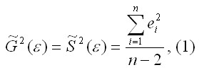
где n – это объём выборочной совокупности;
еi– остатки регрессионной модели:

Для линейной модели множественной регрессии несмещённая оценка дисперсии случайной ошибки рассчитывается по формуле:
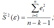
где k – число оцениваемых параметров модели регрессии.
Оценка матрицы ковариаций случайных ошибок Cov(?) будет являться оценочная матрица ковариаций:
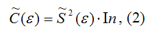
где In – единичная матрица.
Оценка дисперсии случайной ошибки модели регрессии распределена по ?2(хи-квадрат) закону распределения с (n-k-1) степенями свободы.
Для доказательства несмещённости оценки дисперсии случайной ошибки модели регрессии необходимо доказать справедливость равенства

Доказательство. Примем без доказательства справедливость следующих равенств:
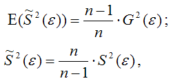
где G2(?) – генеральная дисперсия случайной ошибки;
S2(?) – выборочная дисперсия случайной ошибки;

– выборочная оценка дисперсии случайной ошибки.
Тогда:

т. е.
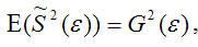
что и требовалось доказать.
Следовательно, выборочная оценка дисперсии случайной ошибки

является несмещённой оценкой генеральной дисперсии случайной ошибки модели регрессии G2(?).
При условии извлечения из генеральной совокупности нескольких выборок одинакового объёма n и при одинаковых значениях объясняющих переменных х, наблюдаемые значения зависимой переменной у будут случайным образом колебаться за счёт случайного характера случайной компоненты ?. Отсюда можно сделать вывод, что будут варьироваться и зависеть от значений переменной у значения оценок коэффициентов регрессии и оценка дисперсии случайной ошибки модели регрессии.
Для иллюстрации данного утверждения докажем зависимость значения МНК-оценки

от величины случайной ошибки ?.
МНК-оценка коэффициента ?1 модели регрессии определяется по формуле:
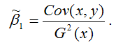
В связи с тем, что переменная у зависит от случайной компоненты ? (yi=?0+?1xi+?i), то ковариация между зависимой переменной у и независимой переменной х может быть представлена следующим образом:

Для дальнейших преобразования используются свойства ковариации:
1) ковариация между переменной х и константой С равна нулю: Cov(x,C)=0, C=const;
2) ковариация переменной х с самой собой равна дисперсии этой переменной: Cov(x,x)=G2(x).
Исходя из указанных свойств ковариации, справедливы следующие равенства:
Cov(x,?0)=0 (?0=const);
Cov(x, ?1x)= ?1*Cov(x,x)= ?1*G2(x).
Следовательно, ковариация между зависимой и независимой переменными Cov(x,y) может быть записана как:
Cov(x,y)= ?1G2(x)+Cov(x,?).
В результате МНК-оценка коэффициента ?1 модели регрессии примет вид:

Таким образом, МНК-оценка

может быть представлена как сумма двух компонент:
1) константы ?1, т. е. истинного значения коэффициента;
2) случайной ошибки Cov(x,?), вызывающей вариацию коэффициента модели регрессии.
Однако на практике подобное разложение МНК-оценки невозможно, потому что истинные значения коэффициентов модели регрессии и значения случайной ошибки являются неизвестными. Теоретически данное разложение можно использовать при изучении статистических свойств МНК-оценок.
Аналогично доказывается, что МНК-оценка

коэффициента модели регрессии и несмещённая оценка дисперсии случайной ошибки

могут быть представлены как сумма постоянной составляющей (константы) и случайной компоненты, зависящей от ошибки модели регрессии ?.
Данный текст является ознакомительным фрагментом.
Читайте также
11. Критерии оценки неизвестных коэффициентов модели регрессии
11. Критерии оценки неизвестных коэффициентов модели регрессии
В ходе регрессионного анализа была подобрана форма связи, которая наилучшим образом отражает зависимость результативной переменной у от факторной переменной х:y=f(x).Необходимо оценить неизвестные
14. Оценка коэффициентов модели парной регрессии с помощью выборочного коэффициента регрессии
14. Оценка коэффициентов модели парной регрессии с помощью выборочного коэффициента регрессии
Помимо метода наименьших квадратов, с помощью которого в большинстве случаев определяются неизвестные параметры модели регрессии, в случае линейной модели парной регрессии
18. Характеристика качества модели регрессии
18. Характеристика качества модели регрессии
Качеством модели регрессии называется адекватность построенной модели исходным (наблюдаемым) данным.Для оценки качества модели регрессии используются специальные показатели.Качество линейной модели парной регрессии
22. Проверка гипотезы о значимости коэффициентов модели парной регрессии
22. Проверка гипотезы о значимости коэффициентов модели парной регрессии
Проверкой статистической гипотезы о значимости отдельных параметров модели называется проверка предположения о том, что данные параметры значимо отличаются от нуля.Необходимость проверки
25. Точечный и интервальный прогнозы для модели парной регрессии
25. Точечный и интервальный прогнозы для модели парной регрессии
Одна из задач эконометрического моделирования заключается в прогнозировании поведения исследуемого явления или процесса в будущем. В большинстве случаев данная задача решается на основе регрессионных
32. Построение частных коэффициентов корреляции для модели множественной регрессии через показатель остаточной дисперсии и коэффициент множественной детерминации
32. Построение частных коэффициентов корреляции для модели множественной регрессии через показатель остаточной дисперсии и коэффициент множественной детерминации
Помимо рекуррентных формул, которые используются для построения частных коэффициентов корреляции для
35. Проверка гипотезы о значимости коэффициентов регрессии и модели множественной регрессии в целом
35. Проверка гипотезы о значимости коэффициентов регрессии и модели множественной регрессии в целом
Проверка значимости коэффициентов регрессии означает проверку основной гипотезы об их значимом отличии от нуля.Основная гипотеза состоит в предположении о незначимости
39. Модели регрессии, нелинейные по факторным переменным
39. Модели регрессии, нелинейные по факторным переменным
При исследовании социально-экономических явлений и процессов далеко не все зависимости можно описать с помощью линейной связи. Поэтому в эконометрическом моделировании широко используется класс нелинейных
40. Модели регрессии, нелинейные по оцениваемым коэффициентам
40. Модели регрессии, нелинейные по оцениваемым коэффициентам
Нелинейными по оцениваемым параметрам моделями регрессииназываются модели, в которых результативная переменная yi нелинейно зависит от коэффициентов модели ?0…?n.К моделям регрессии, нелинейными по
41. Модели регрессии с точками разрыва
41. Модели регрессии с точками разрыва
Определение. Моделями регрессии с точками разрыва называются модели, которые нельзя привести к линейной форме, т. е. внутренне нелинейные модели регрессии.Модели регрессии делятся на два класса:1) кусочно-линейные модели регрессии;2)
44. Методы нелинейного оценивания коэффициентов модели регрессии
44. Методы нелинейного оценивания коэффициентов модели регрессии
Функцией потерь или ошибок называется функционал вида
Также в качестве функции потерь может быть использована сумма модулей отклонений наблюдаемых значений результативного признака у от теоретических
46. Проверка гипотезы о значимости нелинейной модели регрессии. Проверка гипотезы о линейной зависимости между переменными модели регрессии
46. Проверка гипотезы о значимости нелинейной модели регрессии. Проверка гипотезы о линейной зависимости между переменными модели регрессии
На нелинейные модели регрессии, которые являются внутренне линейными, т. е. сводимыми к линейному виду, распространяются все
57. Гетероскедастичность остатков модели регрессии
57. Гетероскедастичность остатков модели регрессии
Случайной ошибкой называется отклонение в линейной модели множественной регрессии:?i=yi–?0–?1x1i–…–?mxmiВ связи с тем, что величина случайной ошибки модели регрессии является неизвестной величиной, рассчитывается
60. Устранение гетероскедастичности остатков модели регрессии
60. Устранение гетероскедастичности остатков модели регрессии
Существует множество методов устранения гетероскедастичности остатков модели регрессии. Рассмотрим некоторые из них.Наиболее простым методом устранения гетероскедастичности остатков модели регрессии
63. Устранение автокорреляции остатков модели регрессии
63. Устранение автокорреляции остатков модели регрессии
В связи с тем, что наличие в модели регрессии автокорреляции между остатками модели может привести к негативным результатам всего процесса оценивания неизвестных коэффициентов модели, автокорреляция остатков
67. Модели регрессии с переменной структурой. Фиктивные переменные
67. Модели регрессии с переменной структурой. Фиктивные переменные
При построении модели регрессии может возникнуть ситуация, когда в неё необходимо включить не только количественные, но и качественные переменные (например, возраст, образование, пол, расовую
Обобщим
КЛММР вида (3.1). Пусть по-прежнему мы
располагаем выборочными наблюдениями
над k
переменными Yi
и
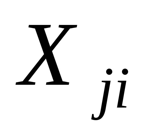 ,j=1,…,
k,
i=1,2,…,n
и строим
регрессию:
 (4.3)
(4.3)
Откажемся
от предположения КЛММР о некоррелированности
и гомоскедастичности случайной ошибки
(3.3). То есть относительно переменных
модели в уравнении (4.3) примем следующие
основные гипотезы:
E(ui)=0;
(4.4)
 (4.5)
(4.5)
X1,
X3,
…, Xk
– неслучайные переменные; (4.6)
Не должно существовать
строгой линейной
зависимости
между переменными X1,
X3,
…, Xk.
(4.7)
Суть
гипотезы (4.5) в том, что все случайные
ошибки ui
имеют непостоянную дисперсию, то есть
не выполняется условие гомоскедастичности
дисперсии – имеет место гетероскедастичность
дисперсии
ошибок. Кроме того, ковариации остатков
могут быть произвольными и отличными
от нуля (вторая строчка соотношения
(4.5)).
Модель
вида (4.3)-(4-7) называется обобщенной
линейной моделью множественной регрессии
(ОЛММР).
Отличие ОЛММР от КЛММР состоит в изменении
предположений о поведении случайной
ошибки (4.5).
К
ОЛММР может быть применен метод наименьших
квадратов, однако (3.6) оказывается
неприменимой к модели (4.3)-(4-7) в силу
потери свойства оптимальности оценок.
Но МНК к ОЛММР может быть применен.
Критерий
минимизации суммы квадратов ошибок МНК
в силу условия (4.5) заменяется на другой
– минимизация обобщенной суммы квадратов
отклонений (с учетом ненулевых ковариаций
случайной ошибки для разных наблюдений
и непостоянной дисперсии ошибки) и
соответственно усложняется вид системы
уравнений для определения оценок
коэффициентов по сравнению с системой
(3.6) для МНК. После решения полученной
системы линейных алгебраических
уравнений получим линейные несмещенные
оценки коэффициентов ОЛММР, которые
будут эффективными. Указанный метод
получения оценок называется обобщенным
методом наименьших квадратов (ОМНК) или
методом Айткена.
Обозначим6:
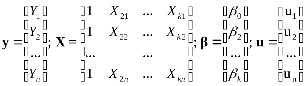 ;
;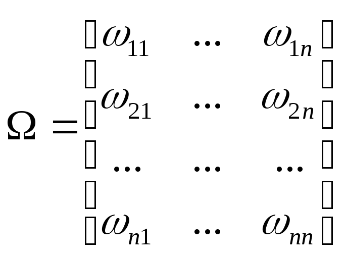 .
.
Тогда
модель (4.3)-(4.7) запишется в матричном
виде:
y=X+u,
при
условиях
E(u)=0;
E(uuT)=2;
X
– не из случайных чисел;
rank(X)=k+1<n.
Оценки
МНК получаются по формуле
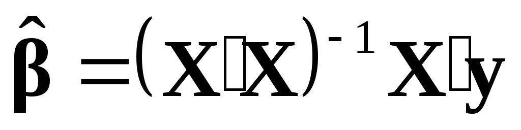 .
.
Оценки ОМНК получаются по формуле .
.
Подчеркнем,
что для применения ОМНК в (4.5) необходимо
знать значения в правой части равенства
(в частности элементы матрицы ),
что на практике случается крайне редко.
Поэтому каким-либо способом оценивают
величины
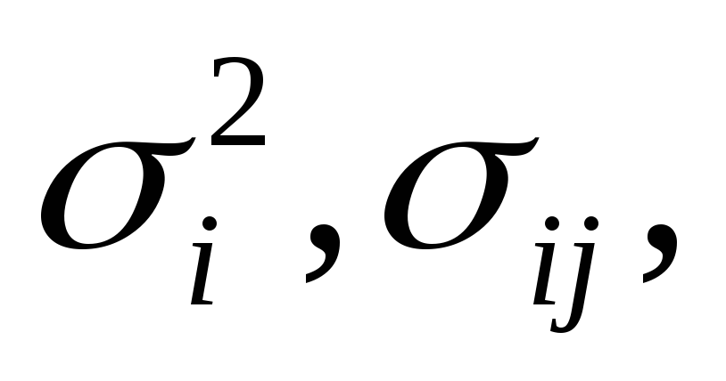 i,
i,
j=1,…,n.
А затем используют эти оценки в расчетах
коэффициентов модели. Этот подход
составляет суть так называемого
доступного
обобщенного метода наименьших квадратов.
Конкретные способы оценки неизвестных
ковариаций будут рассмотрены ниже.
4.3 Линейная модель множественной регрессии
с
гетероскедастичными остатками
Довольно
часто при построении регрессии
анализируемые объекты неоднородны,
например, при исследовании структуры
потребления домохозяйств естественно
ожидать, что колебания в структуре будут
выше для богатых, чем для бедных
домохозяйств. В этой ситуации предположение
(3.3) о постоянстве
дисперсии случайной
ошибки (имеется в виду возможное поведение
случайного члена до того, как сделана
выборка) оказывается не соответствующим
действительности. В случаях, когда
дисперсия u
одинакова
в каждый момент времени или для каждого
значения X,
существуют определенные ограничения
(в некоторой полосе) для расположения
точек на графике X
и Y,
согласно которым отчетливой тенденции
к увеличению или уменьшению дисперсии
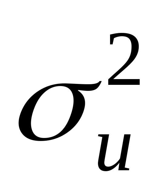 по мере ростаX
не наблюдается.
На
рис. 4.1 приводятся примеры изменения
разброса (гетероскедастичности) случайной
ошибки регрессии.
На
рис. 4.1а изображена ситуация, когда
значения дисперсии
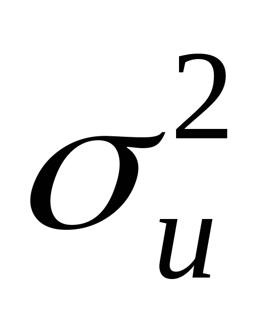 растут по мере увеличения значений
регрессораX.
На рис. 4.1б дисперсия ошибки достигает
максимальной величины при средних
значениях X,
уменьшаясь по мере приближения к крайним
значениям. Наконец, на рис. 4.1в дисперсия
ошибки оказывается наибольшей при малых
значениях X,
быстро уменьшается и становится
однородной по мере увеличения независимой
переменной X.
Y
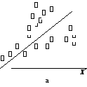

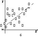
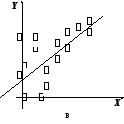
Рис.
4.1. Примеры гетероскедастичности
Гетероскедастичность
дисперсии
случайного члена означает, что
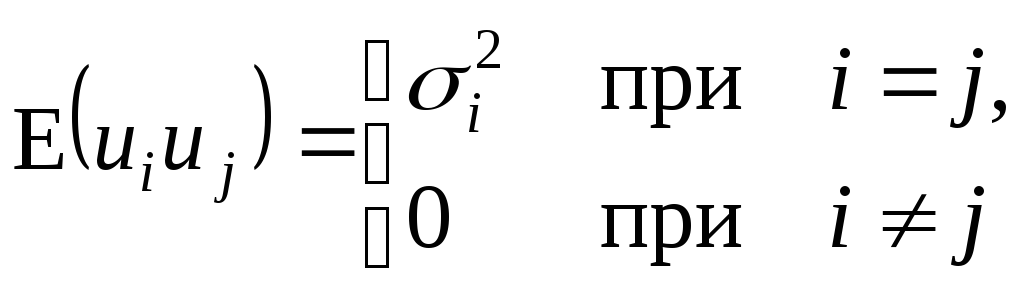 ,
,
(4.8)
т.е.
нарушается предположение (3.3) в КЛММР,
и мы должны рассматривать ОЛММР с нулевой
ковариацией случайных ошибок (ср. (4.5) и
(4.8)).
Основные
последствия гетероскедастичности
проявляются в получении неэффективных
оценок МНК и занижении стандартных
ошибок коэффициентов регрессии, что
завышает t-статистику
и дает неправильное представление о
точности уравнения регрессии.
Поэтому
для оценивания регрессии с гетероскедастичными
случайными ошибками применяется ОМНК.
Предположим,
что нам известны значения величин
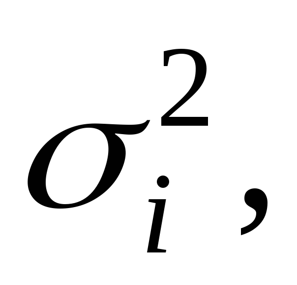 i
i
=1,…,n.
Тогда уравнение (4.3) разделим на i:
 ,
,
и
получим регрессию с постоянной
(гомоскедастичной) дисперсией случайного
члена, действительно
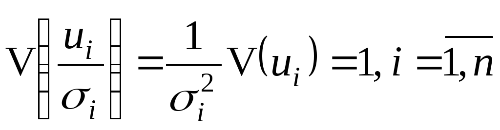 .
.
Для
получения оценок неизвестных дисперсий
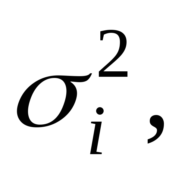 i
i
=1,…,n
будем
предполагать, что они пропорциональны
некоторым числам, т.е.
 ,
,
где 2
– некоторая константа.
Принимая
различные гипотезы относительно
характера гетероскедастичности, будем
иметь соответствующие значения i.
Если
дисперсия случайного члена пропорциональна
квадрату регрессора X,
так что
 ,
,
то
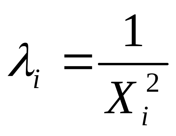 ,i
,i
=1,…,n.
Если
дисперсия случайного члена пропорциональна
X,
так что
 ,
,
то
 ,i
,i
=1,…,n.
Например, для случая одной объясняющей
переменной имеем в этом случае систему
уравнений ОМНК вида:
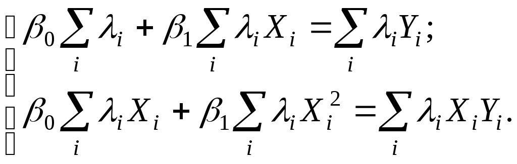
Поскольку значения
i,i=1,…,nявляются фактически весами, которые
устраняют неоднородность дисперсии,
то ОМНК для системы с гетероскедастичностью
часто называютметодом взвешенных
наименьших квадратов.
Существуют также
и другие методы коррекции модели на
гетероскедастичность, в частности
состоятельное оценивание стандартных
ошибок. Известны способы коррекции
стандартных ошибок Уайта и Невье-Веста
[5, с. 144-146].
О проверке выборки
на гомоскедастичность.
Рассмотрим вопрос
тестирования выборки на наличие
гомоскедастичности. Возможности такой
проверки зависят от природы исходных
данных.
Если
имеется обширная выборка, то можно
воспользоваться стандартным критерием
однородности дисперсии Бартлетта.
Расчленяя
выборку на m
независимых групп (каждой из них
соответствует единственное значение
переменной X),
вычислим величины:
 ,
,
причем
ni=n,
здесь ni
— число наблюдений в i
группе,
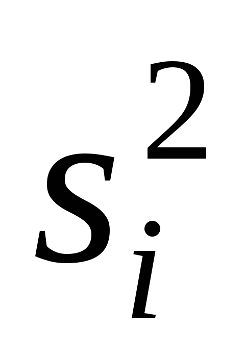 — дисперсия ошибки вi
группе. Величина Q1/Q2
будет приближенно удовлетворять
распределению 2
с (m-1)
степенями свободы. Если вычисленное по
выборке значение 2
меньше критического, то гипотеза об
однородности выборочной дисперсии
принимается, в противном случае
отклоняется.
В
случаях малого количества наблюдений
в выборке, когда группировка данных
невозможна, используется тест
Голдфелда и Куандта.
Он предусматривает осуществление
следующих шагов:
1. Упорядочить
наблюдения по убыванию той независимой
переменной, относительно которой есть
подозрение на гетероскедастичность.
2.
Опустить v
наблюдений, оказавшихся в центре (v
должно быть примерно равно четверти
общего количества наблюдений n).
3.
Оценить отдельно обыкновенным методом
наименьших квадратов регрессии на
первых (n—v)/2
наблюдениях и на последних (n—v)/2
наблюдениях при условии, что (n—v)/2
больше числа оцениваемых параметров
k.
4.
Пусть e1
и e2
— суммы квадратов остатков от первой и
второй регрессий соответственно. Тогда
статистика Q=e1/e2
будет удовлетворять F
— распределению с ((n—v-2k)/2;
(n—v-2k)/2)
степенями свободы. При Q
< F
гипотеза об однородности выборочной
дисперсии принимается, в противном
случае (с ростом величины Q)
отклоняется.
Очевидно,
что решающим для этого теста является
выбор величины v.
Слишком большое значение v
уменьшает надежность теста. Экспериментально
авторами теста установлено, что для
одной объясняющей переменной оптимальное
v=8
при n=30
и v=16
при n=60.
Кроме
перечисленных, могут использоваться
тесты на гетероскедастичность Уайта,
Бреуша-Пагана и др.
Пример.
Проверим по критерию Бартлетта данные
из примера 1 раздела 3. Будем иметь табл.
4.1. В табл. 4.1 учтено, что среднее значение
ei
равно 0, а значит,
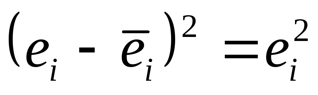 .
.
Примем m=2.
Тогда:
Q1=20ln(10/20167,41
+ 10/2059,69)
(10ln(167,41)+10ln(59,69))=2,55;
Q2=1+1/3(1/10+1/10-1/20)=1,05;
Q1/Q2=2,43.
При
одной степени свободы критическое
значение 2
при 5% уровне значимости равно 3,84, а
следовательно, гипотеза об однородности
выборочной дисперсии принимается.
Для
тех же данных применим тест Гольдфельда
и Куандта. В нашем случае число объясняющих
переменных k=2,
количество исходных данных в выборке
n=20.
Упорядочим наблюдения по убыванию
независимой переменной X2
– расстояние перевозки, относительно
которой есть подозрение на
гетероскедастичность. Опустим 4
наблюдения, оказавшихся в центре, т.е.
v=4.
При значении v=4
получим суммы квадратов остатков от
первой и второй регрессий соответственно
e1=1167,38
и e2=31,49.
Статистика Q=e1/e2=1167,38/31,49
= 37,07 удовлетворяет F-распределению
с (6; 6) степенями свободы. F0,05(6,
6) = 4,28, Q
> F
и гипотеза об однородности выборочной
дисперсии должна быть отвергнута.
Поскольку
тесты дают противоположные результаты
(что не редкость в эконометрике), то
лучше согласиться с наихудшим вариантом,
т.е. предположить наличие гетероскедастичности
и предпринять соответствующие
корректирующие меры. В частности,
скорректировать стандартные ошибки по
формуле Невье-Веста. В таблице 4.2
представлены результаты регрессии до
корректировки и после корректировки
на гетероскедастичность. Видно, что на
величине коэффициентов регрессии
корректировка на гетероскедастичность
не отражается, а стандартные ошибки и
значения статистик были пересчитаны.
Таблица
4.1
Соседние файлы в предмете [НЕСОРТИРОВАННОЕ]
- #
- #
- #
- #
- #
- #
- #
- #
- #
- #
- #
Линейная регрессия: моделирование и допущения
Перевод
Ссылка на автора

Регрессионный анализ — это мощный статистический процесс для поиска отношений в наборе данных, при этом основное внимание уделяется отношениям между независимыми переменными (предикторами) и зависимой переменной (результатом). Он может быть использован для построения моделей для вывода или прогнозирования. Среди нескольких методов регрессионного анализа, линейная регрессия устанавливает основу и довольно широко используется для несколько реальных приложений,
В этой статье мы рассмотрим построение модели линейной регрессии для вывода. Набор данных, который мы будем использовать, это данные о страховых сборах, полученные из Kaggle, Этот набор данных состоит из 1338 наблюдений и 7 столбцов: возраст, пол, bmi, дети, курильщик, регион и сборы.
Ключевые вопросы, которые мы будем задавать:
- Существует ли связь между медицинскими расходами и другими переменными в наборе данных?
- Насколько верна модель, которую мы построили?
- Что мы можем сделать, чтобы улучшить модель?

Начнем с импорта основных необходимых библиотек и данных:
library(magrittr)
library(car)
library(broom)
library(ggplot2)fileName <- './input/medicalCost/insurance.csv'insurance <- read.csv(fileName)
summary(insurance)

Некоторые простые наблюдения, которые можно сделать из резюме:
- Возраст участников варьируется от 18 до 64 лет.
- Около 49,48% участников составляют женщины.
- Bmi участников колеблется от 15,96 до 53,13.
- Только 20,48% участников являются курильщиками.
Давайте начнем с построения линейной модели. Вместо простой линейной регрессии, где у вас есть один предиктор и один результат, мы будем использовать множественную линейную регрессию, где у вас есть более одного предиктора и один результат.
Множественная линейная регрессия следует формуле:

Коэффициенты в этом линейном уравнении обозначают величину аддитивного отношения между предиктором и откликом. Проще говоря, если все остальное зафиксировать, изменение единицы в x1 приведет к изменению β1 в результате, и так далее.
Есть ли связь между медицинскими расходами и предикторами?
Наш первый шаг — выяснить, есть ли связь между результатом и предикторами.
Нулевая гипотеза состояла бы в том, что нет никакой связи между какими-либо предикторами и ответом, что можно проверить путем вычисления F статистика, Значение p статистики F можно использовать для определения, можно ли отклонить нулевую гипотезу или нет.
Мы начнем с подбора модели множественной линейной регрессии с использованием всех предикторов:
lm.fit <- lm(formula = charges~., data = insurance)
#Here '.' means we are using all the predictors in the dataset.

summary(lm.fit)

Высокое значение F-статистики с очень низким p-значением (<2,2e-16) подразумевает, что нулевая гипотеза может быть отклонена. Это означает, что существует потенциальная связь между предикторами и результатом.
RSE (Остаточная стандартная ошибка) — это оценка стандартного отклонения неприводимой ошибки (ошибки, которую нельзя уменьшить, даже если мы знали истинную линию регрессии; следовательно, неприводимую). Проще говоря, это среднее отклонение между фактическим результатом и истинной линией регрессии. Большое значение RSE (6062) означает большое отклонение нашей модели от истинной линии регрессии.
R-квадрат (R²) измеряет долю изменчивости в результате, которая может быть объяснена моделью, и является почти всегда между 0 и 1 ; чем выше значение, тем лучше модель способна объяснить изменчивость в результате. Однако увеличение числа предикторов в основном приводит к увеличению значения R² из-за инфляция R-квадрат, Скорректированный R-квадрат регулирует значение R², чтобы избежать этого эффекта. Высокое значение скорректированного R² (0,7494) показывает, что более 74% отклонений в данных объясняется моделью.
Std. Ошибка дает нам среднюю величину, на которую оценочный коэффициент предиктора отличается от фактического коэффициента предиктора. Он может быть использован для вычисления доверительного интервала предполагаемого коэффициента, который мы увидим позже.
т значениепредиктора говорит нам, сколько стандартных отклонений его расчетный коэффициент от 0.Pr (> | t |)для предиктора — это значение p для оцененного коэффициента регрессии, которое аналогично тому, как сказать, какова вероятность увидеть значение t для коэффициента регрессии. Очень низкое значение p (<0,05) для предиктора может быть использовано для того, чтобы сделать вывод, что существует связь между предиктором и результатом.
Наш следующий шаг должен быть валидация регрессионного анализа, Это может означать проверку основополагающих допущений модели, проверку структуры модели с разными предикторами, поиск наблюдений, которые не были достаточно хорошо представлены в модели, и многое другое. Мы рассмотрим некоторые из этих методов и предположений.
Какие переменные имеют сильное отношение к медицинским расходам?
Теперь, когда мы определили, что существует связь между предикторами и результатом, наш следующий шаг будет выяснить, все ли или только некоторые из предикторов связаны с результатом
Если мы посмотрим на p-значения оценочных коэффициентов выше, мы увидим, что не все коэффициенты статистически значимы (<0,05). Это означает, что только часть предикторов связана с результатом.
Мы можем посмотреть на отдельные p-значения для выбора переменных. Это не может быть проблемой, когда количество предикторов (7) довольно мало по сравнению с количеством наблюдений (1338). Однако этот метод не будет работать, когда число предикторов больше числа наблюдений из-за проблема множественного тестирования, Лучший способ выбора предикторов выбор функции / переменной методы, такие как прямой выбор, обратный выбор или смешанный выбор.
Прежде чем перейти к выбору объектов, используя любой из этих методов, давайте попробуем линейную регрессию, используя объекты только со значимыми значениями p.
lm.fit.sel <- lm(charges~age+bmi+children+smoker+region,
    data = insurance)
Мы сравним это с смешанный выбор, который является комбинацией прямого и обратного выбора. Это можно сделать в R, используяstepAIC ()функция, которая использует Информационный критерий Акайке (AIC), чтобы выбрать лучшую модель из нескольких моделей.
#selecting direction = "both" for mixed selection
step.lm.fit <- MASS::stepAIC(lm.fit, direction = "both",
    trace = FALSE)
Давайте сравним две модели:
step.lm.fit$call
lm.fit.sel$call

Модель, заданная пошаговым отбором, такая же, как модель, которую мы получили, выбрав предикторы со значительными значениями p (работает в этом случае)
Есть ли мультиколлинеарные особенности?
Мультиколлинеарность в множественной регрессии — это явление, при котором два или более предиктора тесно связаны друг с другом, и, следовательно, один предиктор может использоваться для прогнозирования значения другого. Проблема с мультиколлинеарностью состоит в том, что это может затруднить оценку индивидуальных эффектов предикторов на результат.
Мультиколлинеарность может быть обнаружена с использованием дисперсионного фактора инфляции (VIF). VIF любого предиктора — это отношение дисперсии его оценочного коэффициента в полной модели к дисперсии его оценочного коэффициента, когда он подходит для результата только сам по себе (как в простой линейной регрессии). VIF 1 указывает на отсутствие мультиколлинеарности. Обычно значение VIF выше 5 или 10 принимается как показатель мультиколлинеарности. Самый простой способ избавиться от мультиколлинеарности в этом случае — отказаться от предиктора с высоким значением VIF.
vif(step.lm.fit) %>%
    knitr::kable()

Ни один из предикторов в нашем случае не имеет высокого значения VIF. Следовательно, нам не нужно беспокоиться о мультиколлинеарности в нашем случае.

Являются ли отношения линейными?
Применяя линейную регрессию, мы предполагаем, что существует линейная связь между предикторами и результатом. Если исходные отношения довольно далеки от линейных, то большинство сделанных нами выводов будет сомнительным.
Нелинейность модели может быть определена с использованием остаточного графика подгоночных значений по отношению к остаточным значениям. остаточный для любого наблюдения — это разница между фактическим результатом и соответствующим результатом в соответствии с моделью. Наличие шаблона на остаточном графике будет означать проблему с линейным допущением модели.
#type = "rstandard" draws a plot for standardized residualsresidualPlot(step.lm.fit, type = "rstandard")

Синяя линия представляет плавный узор между установленными значениями и стандартными невязками. Кривая в нашем случае обозначает небольшую нелинейность в наших данных.
Нелинейность можно дополнительно изучить, посмотрев на Остаточные участки (Графики ЧР).
ceresPlots(step.lm.fit)

Розовая линия (линия остатка) моделируется для связи между предиктором и остатками. Синяя пунктирная линия (линия компонента) предназначена для линии наилучшего соответствия. Значительная разница между двумя линиями для предиктора подразумевает, что предиктор и результат не имеют линейных отношений.
Этот вид несоответствия можно увидеть на графике CR дляиндекс массы тела, Одним из методов исправления этого является введение нелинейного преобразования предикторов модели. Давайте попробуем добавить нелинейное преобразованиеиндекс массы телак модели.
#update() can be used to update an existing model with new requirementsstep.lm.fit.new <- update(step.lm.fit, .~.+I(bmi^1.25)) ceresPlots(step.lm.fit.new)

График CR bmi больше не имеет разницы между остаточной линией и компонентной линией.
Мы можем использовать ANOVA, чтобы проверить, значительно ли новая модель лучше предыдущей. Низкое значение p (<0,05) для новой модели будет означать, что мы можем сделать вывод, что она лучше, чем в предыдущей модели:
anova(step.lm.fit, step.lm.fit.new, test = "F")

Поскольку модель с нелинейным преобразованиеминдекс массы телаимеет достаточно низкое значение p (<0,05), можно сделать вывод, что оно лучше, чем в предыдущей модели, хотя значение p незначительно.
Давайте посмотрим на остаточный сюжет этой новой модели.
residualPlot(step.lm.fit.new, type = "rstandard")

Глядя на остаточный график новой модели, не наблюдается больших изменений в общей структуре стандартных остатков.

Другим методом решения проблемы нелинейности является введение взаимодействие между некоторыми предикторами. Человек, который курит и имеет высокий BMI, может иметь более высокие расходы по сравнению с человеком, который имеет более низкий BMI и является некурящим Давайте обновим модель, чтобы ввести взаимодействие междуиндекс массы телаа такжекурильщики посмотреть, если это имеет значение:
lm.fit1 <- update(step.lm.fit.new, ~ .+bmi*smoker)residualPlot(lm.fit1, type = "rstandard", id=TRUE)

anova(step.lm.fit.new, lm.fit1, test = "F")

Мало того, что отношение становится более линейным с меньшим появлением рисунка на остаточном графике, новая модель значительно лучше, чем предыдущая модель (без взаимодействий), что можно увидеть при значении p (<2.2e-16).
#checking the value of adjusted r-squared of new model summary(lm.fit1)$adj.r.squared

Значение R² модели также увеличилось до более чем 0,84.
Непостоянная дисперсия ошибок
Постоянная дисперсия (гомоскедастичность) ошибок — еще одно предположение о модели линейной регрессии. Термины ошибок могут, например, изменяться со значением переменной отклика в случае непостоянной дисперсии (гетероскедастичности) ошибок. Некоторые из графических методов определения гетероскедастичности — это наличие воронкообразной формы на остаточном графике или наличие кривой на остаточном графике. На приведенном выше графике мы не видим четкой картины.
Статистический способ — это расширение теста Бреуша-Пагана, доступное в R какncvTest ()в пакете машин. Предполагается, что нулевая гипотеза о постоянной дисперсии ошибок отличается от альтернативной гипотезы о том, что дисперсия ошибок изменяется в зависимости от уровня ответа или от линейной комбинации предикторов.
# non-constant error variance test
ncvTest(lm.fit1)

Очень низкое значение p (~ 0,000023) означает, что нулевая гипотеза может быть отклонена. Другими словами, существует высокая вероятность того, что ошибки имеют непостоянную дисперсию.
Одним из методов решения этой проблемы является преобразование переменной результата.
yTransformer <- 0.8
trans.lm.fit <- update(lm.fit1, charges^yTransformer~.)# non-constant error variance test
ncvTest(trans.lm.fit)

residualPlot(trans.lm.fit, type = "rstandard", id=T)

Значение p, равное ~ 0,94, подразумевает, что мы не можем отвергнуть нулевую гипотезу о постоянной дисперсии членов ошибки. Однако наблюдается небольшое увеличение нелинейности модели, что видно на остаточном графике. Это может быть исправлено в дальнейшем, глядя на отношения между отдельными предикторами и результатами.
Соотношение условий ошибок
Важным допущением модели линейной регрессии является то, что члены последовательных ошибок некоррелированы. Стандартные ошибки оцененных коэффициентов регрессии рассчитываются на основе этого предположения. Если последовательные члены ошибки коррелируют, стандартные ошибки оцененных коэффициентов регрессии могут быть намного больше.
Мы можем проверить автокорреляцию ошибок с помощью Тест Дурбина-Ватсона, Нулевая гипотеза состоит в том, что последовательные ошибки не имеют автокорреляции.
set.seed(1)# Test for Autocorrelated Errors
durbinWatsonTest(trans.lm.fit, max.lag = 5, reps=1000)

Значение р ни для одного из 5 лагов не меньше 0,05. Следовательно, мы не можем отвергнуть нулевую гипотезу о том, что последовательные ошибки не коррелированы, заключив, что последовательные ошибки не зависят друг от друга.
Интерпретации
Давайте посмотрим на фактические расходы в сравнении с установленными значениями для окончательной модели и сравним ее с результатами исходной модели. Функция для построения fit_vs_actual, которая будет использоваться перед следующим блоком, Вот:
#fitted values of initial modelfitted_init <- predict(lm.fit, insurance,
    interval = "confidence") %>%
    tidy()
g1 <- fitted_vs_actual(fitted_init, "Initial Model")#fitted values of final modelfitted_final <- predict(trans.lm.fit, insurance,
    interval = "confidence")^(1/yTransformer) %>%
    tidy()
g2 <- fitted_vs_actual(fitted_final, "Final Model")#creating the two plots side-by-side
gridExtra::grid.arrange(g1,g2, ncol = 2)

Первоначальная модель способна приблизить фактические расходы ниже 17 000 долларов США, но, поскольку фактические расходы превышают 20 000 долларов США, разрыв между фактическими расходами и установленными значениями продолжает увеличиваться. В соответствии с первоначальной моделью, фактические расходы около 50 000 долларов США устанавливаются примерно на уровне 40 000 долларов США или ниже, и этот разрыв продолжает увеличиваться.
Для сравнения, установленные значения в новой модели намного ближе к фактическим расходам, хотя есть еще много изменений, не объясняемых этой моделью. Это все еще значительное улучшение по сравнению с первоначальной моделью.
Мы можем посмотреть на оценочные коэффициенты предикторов и их доверительные интервалы для интерпретации того, как они определяют модель.
confint(trans.lm.fit) %>%
    tidy() %>%
    tibble::add_column(coefficients = trans.lm.fit$coefficients,
        .after = 2) %>%
    knitr::kable()

В приведенной выше таблице X2.5 и X97.5 отмечают нижнюю и верхнюю границы для 95% доверительного интервала коэффициентов регрессии. Они рассчитываются с использованием стандартных ошибок оценочных коэффициентов. В качестве примера длявозрастоценочный коэффициент составляет ~ 33,69, а 95% -ный доверительный интервал находится между ~ 31,56 и ~ 35,83. Это означает, что в соответствии с моделью, сохраняя все остальное фиксированным, увеличение возраста в 1 год приведет к увеличению стоимости обвинений на 33,69 ^ (0,8). (так как мы изменили результат). Тем не менее, это оценка и, следовательно, есть возможность для вариаций. Это изменение объясняется доверительным интервалом, означающим, что примерно в 95% случаев изменение величины зарядов ^ (0,8) будет между 31,56 и 35,83, сохраняя все остальное фиксированным.
Давайте визуализируем эти эффекты, чтобы лучше понять, как предикторы связаны с результатом в соответствии с моделью. Функция для получения эффектов модели на преобразованный результат Вот,
plot_effect('age', 'age') %>%
    ggplot(aes(x = age, y = fit)) +
    theme_bw() +
    geom_line() +
    geom_ribbon(aes(ymin = lower, ymax = upper), alpha = 0.5)

Для среднего значения других предикторов страховые сборы увеличиваются с увеличением возраста. Более интересные эффекты можно увидеть для взаимодействия междуиндекс массы телаа такжекурильщик:
plot_effect('bmi*smoker', 'bmi') %>%
    ggplot(aes(x = x.bmi, y = fit)) +
    facet_wrap(~x.smoker) +
    theme_bw() +
    geom_line() +
    geom_ribbon(aes(ymin = lower, ymax = upper), alpha = 0.5)

Некурящие, независимо от их bmi, имеют в основном низкие страховые взносы для среднего значения других предикторов Курильщики с низким bmi имеют низкие страховые взносы, хотя все еще выше, чем некурящие с любым значением bmi. Более того, по мере того как их bmi увеличивается, страховые сборы курильщиков быстро растут.
Вывод
Модель, которую мы построили, может использоваться для вывода о том, как различные предикторы влияют на результат Это далеко от совершенства. Их по-прежнему наличие нелинейности и непостоянной дисперсии ошибок. Кроме того, выбросы и точки воздействия должны быть проанализированы, чтобы найти лучшую модель. Он не может (и, скорее всего, не даст) аналогичных результатов, когда используется для прогнозирования результата для новых невидимых данных. Чтобы использовать его для прогнозирования, необходимо принять более конкретные меры для обеспечения точности модели, например перекрестную проверку. Это все еще помогает, предоставляя хорошие оценки значимых отношений между предикторами и результатом. Эти оценки могут быть использованы для обобщения данных в более полезной и представительной форме.
Вы можете увидеть оригинальный пост Вот или найди меня на LinkedIn,
источники
- Введение в статистическое обучение, с применением в R. Джеймс Дж., Виттен Д., Хасти Х., Тибширани Р.
- Википедия
- Quick-R
- Статистика Как
- StackExchange
- Переполнение стека