| Error function | |
|---|---|
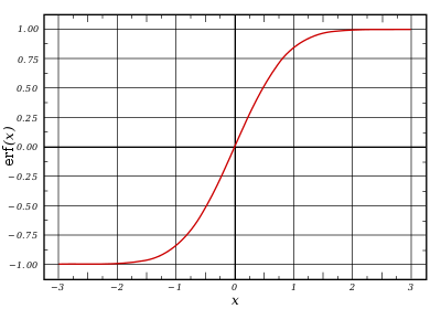
Plot of the error function |
|
| General information | |
| General definition | 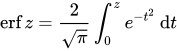 |
| Fields of application | Probability, thermodynamics |
| Domain, Codomain and Image | |
| Domain |  |
| Image |  |
| Basic features | |
| Parity | Odd |
| Specific features | |
| Root | 0 |
| Derivative |  |
| Antiderivative | 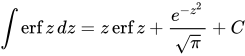 |
| Series definition | |
| Taylor series | 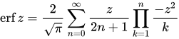 |
In mathematics, the error function (also called the Gauss error function), often denoted by erf, is a complex function of a complex variable defined as:[1]
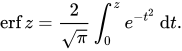
This integral is a special (non-elementary) sigmoid function that occurs often in probability, statistics, and partial differential equations. In many of these applications, the function argument is a real number. If the function argument is real, then the function value is also real.
In statistics, for non-negative values of x, the error function has the following interpretation: for a random variable Y that is normally distributed with mean 0 and standard deviation 1/√2, erf x is the probability that Y falls in the range [−x, x].
Two closely related functions are the complementary error function (erfc) defined as

and the imaginary error function (erfi) defined as

where i is the imaginary unit
Name[edit]
The name «error function» and its abbreviation erf were proposed by J. W. L. Glaisher in 1871 on account of its connection with «the theory of Probability, and notably the theory of Errors.»[2] The error function complement was also discussed by Glaisher in a separate publication in the same year.[3]
For the «law of facility» of errors whose density is given by
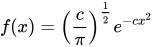
(the normal distribution), Glaisher calculates the probability of an error lying between p and q as:
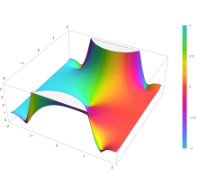
Plot of the error function Erf(z) in the complex plane from -2-2i to 2+2i with colors created with Mathematica 13.1 function ComplexPlot3D

Applications[edit]
When the results of a series of measurements are described by a normal distribution with standard deviation σ and expected value 0, then erf (a/σ √2) is the probability that the error of a single measurement lies between −a and +a, for positive a. This is useful, for example, in determining the bit error rate of a digital communication system.
The error and complementary error functions occur, for example, in solutions of the heat equation when boundary conditions are given by the Heaviside step function.
The error function and its approximations can be used to estimate results that hold with high probability or with low probability. Given a random variable X ~ Norm[μ,σ] (a normal distribution with mean μ and standard deviation σ) and a constant L < μ:
![{displaystyle {begin{aligned}Pr[Xleq L]&={frac {1}{2}}+{frac {1}{2}}operatorname {erf} {frac {L-mu }{{sqrt {2}}sigma }}\&approx Aexp left(-Bleft({frac {L-mu }{sigma }}right)^{2}right)end{aligned}}}](https://wikimedia.org/api/rest_v1/media/math/render/svg/f3cb760eaf336393db9fd0bb12c4465655a27de8)
where A and B are certain numeric constants. If L is sufficiently far from the mean, specifically μ − L ≥ σ√ln k, then:
![{displaystyle Pr[Xleq L]leq Aexp(-Bln {k})={frac {A}{k^{B}}}}](https://wikimedia.org/api/rest_v1/media/math/render/svg/2baadea015e20a45d1034fd88eed861e7fcce178)
so the probability goes to 0 as k → ∞.
The probability for X being in the interval [La, Lb] can be derived as
![{displaystyle {begin{aligned}Pr[L_{a}leq Xleq L_{b}]&=int _{L_{a}}^{L_{b}}{frac {1}{{sqrt {2pi }}sigma }}exp left(-{frac {(x-mu )^{2}}{2sigma ^{2}}}right),mathrm {d} x\&={frac {1}{2}}left(operatorname {erf} {frac {L_{b}-mu }{{sqrt {2}}sigma }}-operatorname {erf} {frac {L_{a}-mu }{{sqrt {2}}sigma }}right).end{aligned}}}](https://wikimedia.org/api/rest_v1/media/math/render/svg/cd2214f0db2c1d36075815825b616501175c6283)
Properties[edit]
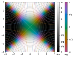
Integrand exp(−z2)

erf z
The property erf (−z) = −erf z means that the error function is an odd function. This directly results from the fact that the integrand e−t2 is an even function (the antiderivative of an even function which is zero at the origin is an odd function and vice versa).
Since the error function is an entire function which takes real numbers to real numbers, for any complex number z:

where z is the complex conjugate of z.
The integrand f = exp(−z2) and f = erf z are shown in the complex z-plane in the figures at right with domain coloring.
The error function at +∞ is exactly 1 (see Gaussian integral). At the real axis, erf z approaches unity at z → +∞ and −1 at z → −∞. At the imaginary axis, it tends to ±i∞.
Taylor series[edit]
The error function is an entire function; it has no singularities (except that at infinity) and its Taylor expansion always converges, but is famously known «[…] for its bad convergence if x > 1.»[4]
The defining integral cannot be evaluated in closed form in terms of elementary functions, but by expanding the integrand e−z2 into its Maclaurin series and integrating term by term, one obtains the error function’s Maclaurin series as:
![{displaystyle {begin{aligned}operatorname {erf} z&={frac {2}{sqrt {pi }}}sum _{n=0}^{infty }{frac {(-1)^{n}z^{2n+1}}{n!(2n+1)}}\[6pt]&={frac {2}{sqrt {pi }}}left(z-{frac {z^{3}}{3}}+{frac {z^{5}}{10}}-{frac {z^{7}}{42}}+{frac {z^{9}}{216}}-cdots right)end{aligned}}}](https://wikimedia.org/api/rest_v1/media/math/render/svg/c80541f305af070bb0510625c584fe1559a0cd2c)
which holds for every complex number z. The denominator terms are sequence A007680 in the OEIS.
For iterative calculation of the above series, the following alternative formulation may be useful:
![{displaystyle {begin{aligned}operatorname {erf} z&={frac {2}{sqrt {pi }}}sum _{n=0}^{infty }left(zprod _{k=1}^{n}{frac {-(2k-1)z^{2}}{k(2k+1)}}right)\[6pt]&={frac {2}{sqrt {pi }}}sum _{n=0}^{infty }{frac {z}{2n+1}}prod _{k=1}^{n}{frac {-z^{2}}{k}}end{aligned}}}](https://wikimedia.org/api/rest_v1/media/math/render/svg/dca22e8e7dee0297e87a455249c282c6b92fedcb)
because −(2k − 1)z2/k(2k + 1) expresses the multiplier to turn the kth term into the (k + 1)th term (considering z as the first term).
The imaginary error function has a very similar Maclaurin series, which is:
![{displaystyle {begin{aligned}operatorname {erfi} z&={frac {2}{sqrt {pi }}}sum _{n=0}^{infty }{frac {z^{2n+1}}{n!(2n+1)}}\[6pt]&={frac {2}{sqrt {pi }}}left(z+{frac {z^{3}}{3}}+{frac {z^{5}}{10}}+{frac {z^{7}}{42}}+{frac {z^{9}}{216}}+cdots right)end{aligned}}}](https://wikimedia.org/api/rest_v1/media/math/render/svg/2ff91095cd6825137cc951ec0a786db0b7f68fac)
which holds for every complex number z.
Derivative and integral[edit]
The derivative of the error function follows immediately from its definition:
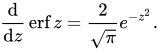
From this, the derivative of the imaginary error function is also immediate:
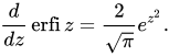
An antiderivative of the error function, obtainable by integration by parts, is
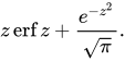
An antiderivative of the imaginary error function, also obtainable by integration by parts, is
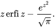
Higher order derivatives are given by

where H are the physicists’ Hermite polynomials.[5]
Bürmann series[edit]
An expansion,[6] which converges more rapidly for all real values of x than a Taylor expansion, is obtained by using Hans Heinrich Bürmann’s theorem:[7]
![{displaystyle {begin{aligned}operatorname {erf} x&={frac {2}{sqrt {pi }}}operatorname {sgn} xcdot {sqrt {1-e^{-x^{2}}}}left(1-{frac {1}{12}}left(1-e^{-x^{2}}right)-{frac {7}{480}}left(1-e^{-x^{2}}right)^{2}-{frac {5}{896}}left(1-e^{-x^{2}}right)^{3}-{frac {787}{276480}}left(1-e^{-x^{2}}right)^{4}-cdots right)\[10pt]&={frac {2}{sqrt {pi }}}operatorname {sgn} xcdot {sqrt {1-e^{-x^{2}}}}left({frac {sqrt {pi }}{2}}+sum _{k=1}^{infty }c_{k}e^{-kx^{2}}right).end{aligned}}}](https://wikimedia.org/api/rest_v1/media/math/render/svg/164e7f029977edb47c83845b04abfe5b2d28b837)
where sgn is the sign function. By keeping only the first two coefficients and choosing c1 = 31/200 and c2 = −341/8000, the resulting approximation shows its largest relative error at x = ±1.3796, where it is less than 0.0036127:

Inverse functions[edit]
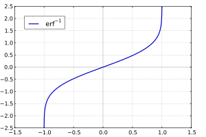
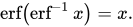
Given a complex number z, there is not a unique complex number w satisfying erf w = z, so a true inverse function would be multivalued. However, for −1 < x < 1, there is a unique real number denoted erf−1 x satisfying
The inverse error function is usually defined with domain (−1,1), and it is restricted to this domain in many computer algebra systems. However, it can be extended to the disk |z| < 1 of the complex plane, using the Maclaurin series
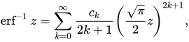
where c0 = 1 and
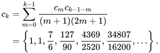
So we have the series expansion (common factors have been canceled from numerators and denominators):

(After cancellation the numerator/denominator fractions are entries OEIS: A092676/OEIS: A092677 in the OEIS; without cancellation the numerator terms are given in entry OEIS: A002067.) The error function’s value at ±∞ is equal to ±1.
For |z| < 1, we have erf(erf−1 z) = z.
The inverse complementary error function is defined as

For real x, there is a unique real number erfi−1 x satisfying erfi(erfi−1 x) = x. The inverse imaginary error function is defined as erfi−1 x.[8]
For any real x, Newton’s method can be used to compute erfi−1 x, and for −1 ≤ x ≤ 1, the following Maclaurin series converges:
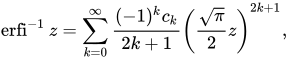
where ck is defined as above.
Asymptotic expansion[edit]
A useful asymptotic expansion of the complementary error function (and therefore also of the error function) for large real x is
![{displaystyle {begin{aligned}operatorname {erfc} x&={frac {e^{-x^{2}}}{x{sqrt {pi }}}}left(1+sum _{n=1}^{infty }(-1)^{n}{frac {1cdot 3cdot 5cdots (2n-1)}{left(2x^{2}right)^{n}}}right)\[6pt]&={frac {e^{-x^{2}}}{x{sqrt {pi }}}}sum _{n=0}^{infty }(-1)^{n}{frac {(2n-1)!!}{left(2x^{2}right)^{n}}},end{aligned}}}](https://wikimedia.org/api/rest_v1/media/math/render/svg/35a11e2e5b22ca898c74f2e913d276c9ac11124a)
where (2n − 1)!! is the double factorial of (2n − 1), which is the product of all odd numbers up to (2n − 1). This series diverges for every finite x, and its meaning as asymptotic expansion is that for any integer N ≥ 1 one has

where the remainder, in Landau notation, is

as x → ∞.
Indeed, the exact value of the remainder is

which follows easily by induction, writing
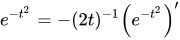
and integrating by parts.
For large enough values of x, only the first few terms of this asymptotic expansion are needed to obtain a good approximation of erfc x (while for not too large values of x, the above Taylor expansion at 0 provides a very fast convergence).
Continued fraction expansion[edit]
A continued fraction expansion of the complementary error function is:[9]
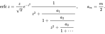
Integral of error function with Gaussian density function[edit]

which appears related to Ng and Geller, formula 13 in section 4.3[10] with a change of variables.
Factorial series[edit]
The inverse factorial series:
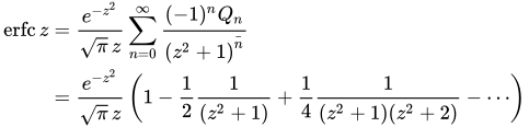
converges for Re(z2) > 0. Here
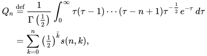
zn denotes the rising factorial, and s(n,k) denotes a signed Stirling number of the first kind.[11][12]
There also exists a representation by an infinite sum containing the double factorial:

Numerical approximations[edit]
Approximation with elementary functions[edit]
- Abramowitz and Stegun give several approximations of varying accuracy (equations 7.1.25–28). This allows one to choose the fastest approximation suitable for a given application. In order of increasing accuracy, they are:
(maximum error: 5×10⁻⁴)
where a1 = 0.278393, a2 = 0.230389, a3 = 0.000972, a4 = 0.078108
(maximum error: 2.5×10⁻⁵)
where p = 0.47047, a1 = 0.3480242, a2 = −0.0958798, a3 = 0.7478556
(maximum error: 3×10⁻⁷)
where a1 = 0.0705230784, a2 = 0.0422820123, a3 = 0.0092705272, a4 = 0.0001520143, a5 = 0.0002765672, a6 = 0.0000430638
(maximum error: 1.5×10⁻⁷)
where p = 0.3275911, a1 = 0.254829592, a2 = −0.284496736, a3 = 1.421413741, a4 = −1.453152027, a5 = 1.061405429
All of these approximations are valid for x ≥ 0. To use these approximations for negative x, use the fact that erf x is an odd function, so erf x = −erf(−x).
- Exponential bounds and a pure exponential approximation for the complementary error function are given by[13]
- The above have been generalized to sums of N exponentials[14] with increasing accuracy in terms of N so that erfc x can be accurately approximated or bounded by 2Q̃(√2x), where
In particular, there is a systematic methodology to solve the numerical coefficients {(an,bn)}N
n = 1 that yield a minimax approximation or bound for the closely related Q-function: Q(x) ≈ Q̃(x), Q(x) ≤ Q̃(x), or Q(x) ≥ Q̃(x) for x ≥ 0. The coefficients {(an,bn)}N
n = 1 for many variations of the exponential approximations and bounds up to N = 25 have been released to open access as a comprehensive dataset.[15] - A tight approximation of the complementary error function for x ∈ [0,∞) is given by Karagiannidis & Lioumpas (2007)[16] who showed for the appropriate choice of parameters {A,B} that
They determined {A,B} = {1.98,1.135}, which gave a good approximation for all x ≥ 0. Alternative coefficients are also available for tailoring accuracy for a specific application or transforming the expression into a tight bound.[17]
- A single-term lower bound is[18]
where the parameter β can be picked to minimize error on the desired interval of approximation.
-
- Another approximation is given by Sergei Winitzki using his «global Padé approximations»:[19][20]: 2–3
where
This is designed to be very accurate in a neighborhood of 0 and a neighborhood of infinity, and the relative error is less than 0.00035 for all real x. Using the alternate value a ≈ 0.147 reduces the maximum relative error to about 0.00013.[21]
This approximation can be inverted to obtain an approximation for the inverse error function:
- An approximation with a maximal error of 1.2×10⁻⁷ for any real argument is:[22]
with
and





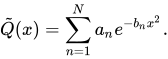
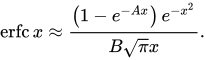


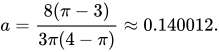

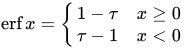

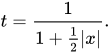
Table of values[edit]
| x | erf x | 1 − erf x |
|---|---|---|
| 0 | 0 | 1 |
| 0.02 | 0.022564575 | 0.977435425 |
| 0.04 | 0.045111106 | 0.954888894 |
| 0.06 | 0.067621594 | 0.932378406 |
| 0.08 | 0.090078126 | 0.909921874 |
| 0.1 | 0.112462916 | 0.887537084 |
| 0.2 | 0.222702589 | 0.777297411 |
| 0.3 | 0.328626759 | 0.671373241 |
| 0.4 | 0.428392355 | 0.571607645 |
| 0.5 | 0.520499878 | 0.479500122 |
| 0.6 | 0.603856091 | 0.396143909 |
| 0.7 | 0.677801194 | 0.322198806 |
| 0.8 | 0.742100965 | 0.257899035 |
| 0.9 | 0.796908212 | 0.203091788 |
| 1 | 0.842700793 | 0.157299207 |
| 1.1 | 0.880205070 | 0.119794930 |
| 1.2 | 0.910313978 | 0.089686022 |
| 1.3 | 0.934007945 | 0.065992055 |
| 1.4 | 0.952285120 | 0.047714880 |
| 1.5 | 0.966105146 | 0.033894854 |
| 1.6 | 0.976348383 | 0.023651617 |
| 1.7 | 0.983790459 | 0.016209541 |
| 1.8 | 0.989090502 | 0.010909498 |
| 1.9 | 0.992790429 | 0.007209571 |
| 2 | 0.995322265 | 0.004677735 |
| 2.1 | 0.997020533 | 0.002979467 |
| 2.2 | 0.998137154 | 0.001862846 |
| 2.3 | 0.998856823 | 0.001143177 |
| 2.4 | 0.999311486 | 0.000688514 |
| 2.5 | 0.999593048 | 0.000406952 |
| 3 | 0.999977910 | 0.000022090 |
| 3.5 | 0.999999257 | 0.000000743 |
[edit]
Complementary error function[edit]
The complementary error function, denoted erfc, is defined as
-
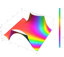
Plot of the complementary error function Erfc(z) in the complex plane from -2-2i to 2+2i with colors created with Mathematica 13.1 function ComplexPlot3D
![{displaystyle {begin{aligned}operatorname {erfc} x&=1-operatorname {erf} x\[5pt]&={frac {2}{sqrt {pi }}}int _{x}^{infty }e^{-t^{2}},mathrm {d} t\[5pt]&=e^{-x^{2}}operatorname {erfcx} x,end{aligned}}}](https://wikimedia.org/api/rest_v1/media/math/render/svg/4acd0062271e2a19c209a02c8cc33d44a28af7cc)
which also defines erfcx, the scaled complementary error function[23] (which can be used instead of erfc to avoid arithmetic underflow[23][24]). Another form of erfc x for x ≥ 0 is known as Craig’s formula, after its discoverer:[25]

This expression is valid only for positive values of x, but it can be used in conjunction with erfc x = 2 − erfc(−x) to obtain erfc(x) for negative values. This form is advantageous in that the range of integration is fixed and finite. An extension of this expression for the erfc of the sum of two non-negative variables is as follows:[26]

Imaginary error function[edit]
The imaginary error function, denoted erfi, is defined as

Plot of the imaginary error function Erfi(z) in the complex plane from -2-2i to 2+2i with colors created with Mathematica 13.1 function ComplexPlot3D
![{displaystyle {begin{aligned}operatorname {erfi} x&=-ioperatorname {erf} ix\[5pt]&={frac {2}{sqrt {pi }}}int _{0}^{x}e^{t^{2}},mathrm {d} t\[5pt]&={frac {2}{sqrt {pi }}}e^{x^{2}}D(x),end{aligned}}}](https://wikimedia.org/api/rest_v1/media/math/render/svg/bfd2dd94cd6d0325224d412f6b5e5ed63ca81d4a)
where D(x) is the Dawson function (which can be used instead of erfi to avoid arithmetic overflow[23]).
Despite the name «imaginary error function», erfi x is real when x is real.
When the error function is evaluated for arbitrary complex arguments z, the resulting complex error function is usually discussed in scaled form as the Faddeeva function:

Cumulative distribution function[edit]
The error function is essentially identical to the standard normal cumulative distribution function, denoted Φ, also named norm(x) by some software languages[citation needed], as they differ only by scaling and translation. Indeed,
-
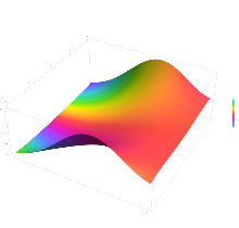
the normal cumulative distribution function plotted in the complex plane
![{displaystyle {begin{aligned}Phi (x)&={frac {1}{sqrt {2pi }}}int _{-infty }^{x}e^{tfrac {-t^{2}}{2}},mathrm {d} t\[6pt]&={frac {1}{2}}left(1+operatorname {erf} {frac {x}{sqrt {2}}}right)\[6pt]&={frac {1}{2}}operatorname {erfc} left(-{frac {x}{sqrt {2}}}right)end{aligned}}}](https://wikimedia.org/api/rest_v1/media/math/render/svg/89a9e9eaaddcd7a91ade15a41b8d1e272d437559)
or rearranged for erf and erfc:
![{displaystyle {begin{aligned}operatorname {erf} (x)&=2Phi left(x{sqrt {2}}right)-1\[6pt]operatorname {erfc} (x)&=2Phi left(-x{sqrt {2}}right)\&=2left(1-Phi left(x{sqrt {2}}right)right).end{aligned}}}](https://wikimedia.org/api/rest_v1/media/math/render/svg/86c84a4d2d79631fe9996e30f1d6c0da3089bfe2)
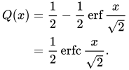
Consequently, the error function is also closely related to the Q-function, which is the tail probability of the standard normal distribution. The Q-function can be expressed in terms of the error function as
The inverse of Φ is known as the normal quantile function, or probit function and may be expressed in terms of the inverse error function as

The standard normal cdf is used more often in probability and statistics, and the error function is used more often in other branches of mathematics.
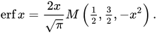
The error function is a special case of the Mittag-Leffler function, and can also be expressed as a confluent hypergeometric function (Kummer’s function):
It has a simple expression in terms of the Fresnel integral.[further explanation needed]
In terms of the regularized gamma function P and the incomplete gamma function,

sgn x is the sign function.
Generalized error functions[edit]

Graph of generalised error functions En(x):
grey curve: E1(x) = 1 − e−x/√π
red curve: E2(x) = erf(x)
green curve: E3(x)
blue curve: E4(x)
gold curve: E5(x).
Some authors discuss the more general functions:[citation needed]

Notable cases are:
- E0(x) is a straight line through the origin: E0(x) = x/e√π
- E2(x) is the error function, erf x.
After division by n!, all the En for odd n look similar (but not identical) to each other. Similarly, the En for even n look similar (but not identical) to each other after a simple division by n!. All generalised error functions for n > 0 look similar on the positive x side of the graph.
These generalised functions can equivalently be expressed for x > 0 using the gamma function and incomplete gamma function:

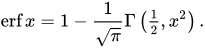
Therefore, we can define the error function in terms of the incomplete gamma function:
Iterated integrals of the complementary error function[edit]
The iterated integrals of the complementary error function are defined by[27]
![{displaystyle {begin{aligned}operatorname {i} ^{n}!operatorname {erfc} z&=int _{z}^{infty }operatorname {i} ^{n-1}!operatorname {erfc} zeta ,mathrm {d} zeta \[6pt]operatorname {i} ^{0}!operatorname {erfc} z&=operatorname {erfc} z\operatorname {i} ^{1}!operatorname {erfc} z&=operatorname {ierfc} z={frac {1}{sqrt {pi }}}e^{-z^{2}}-zoperatorname {erfc} z\operatorname {i} ^{2}!operatorname {erfc} z&={tfrac {1}{4}}left(operatorname {erfc} z-2zoperatorname {ierfc} zright)\end{aligned}}}](https://wikimedia.org/api/rest_v1/media/math/render/svg/c3e7b953efaa4d730a5479bd61a2c378c8f761dc)
The general recurrence formula is

They have the power series
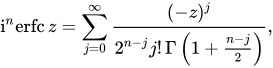
from which follow the symmetry properties

and

Implementations[edit]
As real function of a real argument[edit]
- In Posix-compliant operating systems, the header
math.hshall declare and the mathematical librarylibmshall provide the functionserfanderfc(double precision) as well as their single precision and extended precision counterpartserff,erflanderfcf,erfcl.[28] - The GNU Scientific Library provides
erf,erfc,log(erf), and scaled error functions.[29]
As complex function of a complex argument[edit]
libcerf, numeric C library for complex error functions, provides the complex functionscerf,cerfc,cerfcxand the real functionserfi,erfcxwith approximately 13–14 digits precision, based on the Faddeeva function as implemented in the MIT Faddeeva Package
See also[edit]
[edit]
- Gaussian integral, over the whole real line
- Gaussian function, derivative
- Dawson function, renormalized imaginary error function
- Goodwin–Staton integral
In probability[edit]
- Normal distribution
- Normal cumulative distribution function, a scaled and shifted form of error function
- Probit, the inverse or quantile function of the normal CDF
- Q-function, the tail probability of the normal distribution
References[edit]
- ^ Andrews, Larry C. (1998). Special functions of mathematics for engineers. SPIE Press. p. 110. ISBN 9780819426161.
- ^ Glaisher, James Whitbread Lee (July 1871). «On a class of definite integrals». London, Edinburgh, and Dublin Philosophical Magazine and Journal of Science. 4. 42 (277): 294–302. doi:10.1080/14786447108640568. Retrieved 6 December 2017.
- ^ Glaisher, James Whitbread Lee (September 1871). «On a class of definite integrals. Part II». London, Edinburgh, and Dublin Philosophical Magazine and Journal of Science. 4. 42 (279): 421–436. doi:10.1080/14786447108640600. Retrieved 6 December 2017.
- ^ «A007680 – OEIS». oeis.org. Retrieved 2 April 2020.
- ^ Weisstein, Eric W. «Erf». MathWorld.
- ^ Schöpf, H. M.; Supancic, P. H. (2014). «On Bürmann’s Theorem and Its Application to Problems of Linear and Nonlinear Heat Transfer and Diffusion». The Mathematica Journal. 16. doi:10.3888/tmj.16-11.
- ^ Weisstein, Eric W. «Bürmann’s Theorem». MathWorld.
- ^ Bergsma, Wicher (2006). «On a new correlation coefficient, its orthogonal decomposition and associated tests of independence». arXiv:math/0604627.
- ^ Cuyt, Annie A. M.; Petersen, Vigdis B.; Verdonk, Brigitte; Waadeland, Haakon; Jones, William B. (2008). Handbook of Continued Fractions for Special Functions. Springer-Verlag. ISBN 978-1-4020-6948-2.
- ^ Ng, Edward W.; Geller, Murray (January 1969). «A table of integrals of the Error functions». Journal of Research of the National Bureau of Standards Section B. 73B (1): 1. doi:10.6028/jres.073B.001.
- ^ Schlömilch, Oskar Xavier (1859). «Ueber facultätenreihen». Zeitschrift für Mathematik und Physik (in German). 4: 390–415. Retrieved 4 December 2017.
- ^ Nielson, Niels (1906). Handbuch der Theorie der Gammafunktion (in German). Leipzig: B. G. Teubner. p. 283 Eq. 3. Retrieved 4 December 2017.
- ^ Chiani, M.; Dardari, D.; Simon, M.K. (2003). «New Exponential Bounds and Approximations for the Computation of Error Probability in Fading Channels» (PDF). IEEE Transactions on Wireless Communications. 2 (4): 840–845. CiteSeerX 10.1.1.190.6761. doi:10.1109/TWC.2003.814350.
- ^ Tanash, I.M.; Riihonen, T. (2020). «Global minimax approximations and bounds for the Gaussian Q-function by sums of exponentials». IEEE Transactions on Communications. 68 (10): 6514–6524. arXiv:2007.06939. doi:10.1109/TCOMM.2020.3006902. S2CID 220514754.
- ^ Tanash, I.M.; Riihonen, T. (2020). «Coefficients for Global Minimax Approximations and Bounds for the Gaussian Q-Function by Sums of Exponentials [Data set]». Zenodo. doi:10.5281/zenodo.4112978.
- ^ Karagiannidis, G. K.; Lioumpas, A. S. (2007). «An improved approximation for the Gaussian Q-function» (PDF). IEEE Communications Letters. 11 (8): 644–646. doi:10.1109/LCOMM.2007.070470. S2CID 4043576.
- ^ Tanash, I.M.; Riihonen, T. (2021). «Improved coefficients for the Karagiannidis–Lioumpas approximations and bounds to the Gaussian Q-function». IEEE Communications Letters. 25 (5): 1468–1471. arXiv:2101.07631. doi:10.1109/LCOMM.2021.3052257. S2CID 231639206.
- ^ Chang, Seok-Ho; Cosman, Pamela C.; Milstein, Laurence B. (November 2011). «Chernoff-Type Bounds for the Gaussian Error Function». IEEE Transactions on Communications. 59 (11): 2939–2944. doi:10.1109/TCOMM.2011.072011.100049. S2CID 13636638.
- ^ Winitzki, Sergei (2003). «Uniform approximations for transcendental functions». Computational Science and Its Applications – ICCSA 2003. Lecture Notes in Computer Science. Vol. 2667. Springer, Berlin. pp. 780–789. doi:10.1007/3-540-44839-X_82. ISBN 978-3-540-40155-1.
- ^ Zeng, Caibin; Chen, Yang Cuan (2015). «Global Padé approximations of the generalized Mittag-Leffler function and its inverse». Fractional Calculus and Applied Analysis. 18 (6): 1492–1506. arXiv:1310.5592. doi:10.1515/fca-2015-0086. S2CID 118148950.
Indeed, Winitzki [32] provided the so-called global Padé approximation
- ^ Winitzki, Sergei (6 February 2008). «A handy approximation for the error function and its inverse».
- ^ Numerical Recipes in Fortran 77: The Art of Scientific Computing (ISBN 0-521-43064-X), 1992, page 214, Cambridge University Press.
- ^ a b c Cody, W. J. (March 1993), «Algorithm 715: SPECFUN—A portable FORTRAN package of special function routines and test drivers» (PDF), ACM Trans. Math. Softw., 19 (1): 22–32, CiteSeerX 10.1.1.643.4394, doi:10.1145/151271.151273, S2CID 5621105
- ^ Zaghloul, M. R. (1 March 2007), «On the calculation of the Voigt line profile: a single proper integral with a damped sine integrand», Monthly Notices of the Royal Astronomical Society, 375 (3): 1043–1048, Bibcode:2007MNRAS.375.1043Z, doi:10.1111/j.1365-2966.2006.11377.x
- ^ John W. Craig, A new, simple and exact result for calculating the probability of error for two-dimensional signal constellations Archived 3 April 2012 at the Wayback Machine, Proceedings of the 1991 IEEE Military Communication Conference, vol. 2, pp. 571–575.
- ^ Behnad, Aydin (2020). «A Novel Extension to Craig’s Q-Function Formula and Its Application in Dual-Branch EGC Performance Analysis». IEEE Transactions on Communications. 68 (7): 4117–4125. doi:10.1109/TCOMM.2020.2986209. S2CID 216500014.
- ^ Carslaw, H. S.; Jaeger, J. C. (1959), Conduction of Heat in Solids (2nd ed.), Oxford University Press, ISBN 978-0-19-853368-9, p 484
- ^ https://pubs.opengroup.org/onlinepubs/9699919799/basedefs/math.h.html
- ^ «Special Functions – GSL 2.7 documentation».
Further reading[edit]
- Abramowitz, Milton; Stegun, Irene Ann, eds. (1983) [June 1964]. «Chapter 7». Handbook of Mathematical Functions with Formulas, Graphs, and Mathematical Tables. Applied Mathematics Series. Vol. 55 (Ninth reprint with additional corrections of tenth original printing with corrections (December 1972); first ed.). Washington D.C.; New York: United States Department of Commerce, National Bureau of Standards; Dover Publications. p. 297. ISBN 978-0-486-61272-0. LCCN 64-60036. MR 0167642. LCCN 65-12253.
- Press, William H.; Teukolsky, Saul A.; Vetterling, William T.; Flannery, Brian P. (2007), «Section 6.2. Incomplete Gamma Function and Error Function», Numerical Recipes: The Art of Scientific Computing (3rd ed.), New York: Cambridge University Press, ISBN 978-0-521-88068-8
- Temme, Nico M. (2010), «Error Functions, Dawson’s and Fresnel Integrals», in Olver, Frank W. J.; Lozier, Daniel M.; Boisvert, Ronald F.; Clark, Charles W. (eds.), NIST Handbook of Mathematical Functions, Cambridge University Press, ISBN 978-0-521-19225-5, MR 2723248
External links[edit]
- A Table of Integrals of the Error Functions
| Error function | |
|---|---|
|
Plot of the error function |
|
| General information | |
| General definition | |
| Fields of application | Probability, thermodynamics |
| Domain, Codomain and Image | |
| Domain | |
| Image | |
| Basic features | |
| Parity | Odd |
| Specific features | |
| Root | 0 |
| Derivative | |
| Antiderivative | |
| Series definition | |
| Taylor series | |
In mathematics, the error function (also called the Gauss error function), often denoted by erf, is a complex function of a complex variable defined as:[1]
This integral is a special (non-elementary) sigmoid function that occurs often in probability, statistics, and partial differential equations. In many of these applications, the function argument is a real number. If the function argument is real, then the function value is also real.
In statistics, for non-negative values of x, the error function has the following interpretation: for a random variable Y that is normally distributed with mean 0 and standard deviation 1/√2, erf x is the probability that Y falls in the range [−x, x].
Two closely related functions are the complementary error function (erfc) defined as
and the imaginary error function (erfi) defined as
where i is the imaginary unit
Name[edit]
The name «error function» and its abbreviation erf were proposed by J. W. L. Glaisher in 1871 on account of its connection with «the theory of Probability, and notably the theory of Errors.»[2] The error function complement was also discussed by Glaisher in a separate publication in the same year.[3]
For the «law of facility» of errors whose density is given by
(the normal distribution), Glaisher calculates the probability of an error lying between p and q as:
Plot of the error function Erf(z) in the complex plane from -2-2i to 2+2i with colors created with Mathematica 13.1 function ComplexPlot3D
Applications[edit]
When the results of a series of measurements are described by a normal distribution with standard deviation σ and expected value 0, then erf (a/σ √2) is the probability that the error of a single measurement lies between −a and +a, for positive a. This is useful, for example, in determining the bit error rate of a digital communication system.
The error and complementary error functions occur, for example, in solutions of the heat equation when boundary conditions are given by the Heaviside step function.
The error function and its approximations can be used to estimate results that hold with high probability or with low probability. Given a random variable X ~ Norm[μ,σ] (a normal distribution with mean μ and standard deviation σ) and a constant L < μ:
where A and B are certain numeric constants. If L is sufficiently far from the mean, specifically μ − L ≥ σ√ln k, then:
so the probability goes to 0 as k → ∞.
The probability for X being in the interval [La, Lb] can be derived as
Properties[edit]
Integrand exp(−z2)
erf z
The property erf (−z) = −erf z means that the error function is an odd function. This directly results from the fact that the integrand e−t2 is an even function (the antiderivative of an even function which is zero at the origin is an odd function and vice versa).
Since the error function is an entire function which takes real numbers to real numbers, for any complex number z:
where z is the complex conjugate of z.
The integrand f = exp(−z2) and f = erf z are shown in the complex z-plane in the figures at right with domain coloring.
The error function at +∞ is exactly 1 (see Gaussian integral). At the real axis, erf z approaches unity at z → +∞ and −1 at z → −∞. At the imaginary axis, it tends to ±i∞.
Taylor series[edit]
The error function is an entire function; it has no singularities (except that at infinity) and its Taylor expansion always converges, but is famously known «[…] for its bad convergence if x > 1.»[4]
The defining integral cannot be evaluated in closed form in terms of elementary functions, but by expanding the integrand e−z2 into its Maclaurin series and integrating term by term, one obtains the error function’s Maclaurin series as:
which holds for every complex number z. The denominator terms are sequence A007680 in the OEIS.
For iterative calculation of the above series, the following alternative formulation may be useful:
because −(2k − 1)z2/k(2k + 1) expresses the multiplier to turn the kth term into the (k + 1)th term (considering z as the first term).
The imaginary error function has a very similar Maclaurin series, which is:
which holds for every complex number z.
Derivative and integral[edit]
The derivative of the error function follows immediately from its definition:
From this, the derivative of the imaginary error function is also immediate:
An antiderivative of the error function, obtainable by integration by parts, is
An antiderivative of the imaginary error function, also obtainable by integration by parts, is
Higher order derivatives are given by
where H are the physicists’ Hermite polynomials.[5]
Bürmann series[edit]
An expansion,[6] which converges more rapidly for all real values of x than a Taylor expansion, is obtained by using Hans Heinrich Bürmann’s theorem:[7]
where sgn is the sign function. By keeping only the first two coefficients and choosing c1 = 31/200 and c2 = −341/8000, the resulting approximation shows its largest relative error at x = ±1.3796, where it is less than 0.0036127:
Inverse functions[edit]
Given a complex number z, there is not a unique complex number w satisfying erf w = z, so a true inverse function would be multivalued. However, for −1 < x < 1, there is a unique real number denoted erf−1 x satisfying
The inverse error function is usually defined with domain (−1,1), and it is restricted to this domain in many computer algebra systems. However, it can be extended to the disk |z| < 1 of the complex plane, using the Maclaurin series
where c0 = 1 and
So we have the series expansion (common factors have been canceled from numerators and denominators):
(After cancellation the numerator/denominator fractions are entries OEIS: A092676/OEIS: A092677 in the OEIS; without cancellation the numerator terms are given in entry OEIS: A002067.) The error function’s value at ±∞ is equal to ±1.
For |z| < 1, we have erf(erf−1 z) = z.
The inverse complementary error function is defined as
For real x, there is a unique real number erfi−1 x satisfying erfi(erfi−1 x) = x. The inverse imaginary error function is defined as erfi−1 x.[8]
For any real x, Newton’s method can be used to compute erfi−1 x, and for −1 ≤ x ≤ 1, the following Maclaurin series converges:
where ck is defined as above.
Asymptotic expansion[edit]
A useful asymptotic expansion of the complementary error function (and therefore also of the error function) for large real x is
where (2n − 1)!! is the double factorial of (2n − 1), which is the product of all odd numbers up to (2n − 1). This series diverges for every finite x, and its meaning as asymptotic expansion is that for any integer N ≥ 1 one has
where the remainder, in Landau notation, is
as x → ∞.
Indeed, the exact value of the remainder is
which follows easily by induction, writing
and integrating by parts.
For large enough values of x, only the first few terms of this asymptotic expansion are needed to obtain a good approximation of erfc x (while for not too large values of x, the above Taylor expansion at 0 provides a very fast convergence).
Continued fraction expansion[edit]
A continued fraction expansion of the complementary error function is:[9]
Integral of error function with Gaussian density function[edit]
which appears related to Ng and Geller, formula 13 in section 4.3[10] with a change of variables.
Factorial series[edit]
The inverse factorial series:
converges for Re(z2) > 0. Here
zn denotes the rising factorial, and s(n,k) denotes a signed Stirling number of the first kind.[11][12]
There also exists a representation by an infinite sum containing the double factorial:
Numerical approximations[edit]
Approximation with elementary functions[edit]
- Abramowitz and Stegun give several approximations of varying accuracy (equations 7.1.25–28). This allows one to choose the fastest approximation suitable for a given application. In order of increasing accuracy, they are:
(maximum error: 5×10⁻⁴)
where a1 = 0.278393, a2 = 0.230389, a3 = 0.000972, a4 = 0.078108
(maximum error: 2.5×10⁻⁵)
where p = 0.47047, a1 = 0.3480242, a2 = −0.0958798, a3 = 0.7478556
(maximum error: 3×10⁻⁷)
where a1 = 0.0705230784, a2 = 0.0422820123, a3 = 0.0092705272, a4 = 0.0001520143, a5 = 0.0002765672, a6 = 0.0000430638
(maximum error: 1.5×10⁻⁷)
where p = 0.3275911, a1 = 0.254829592, a2 = −0.284496736, a3 = 1.421413741, a4 = −1.453152027, a5 = 1.061405429
All of these approximations are valid for x ≥ 0. To use these approximations for negative x, use the fact that erf x is an odd function, so erf x = −erf(−x).
- Exponential bounds and a pure exponential approximation for the complementary error function are given by[13]
- The above have been generalized to sums of N exponentials[14] with increasing accuracy in terms of N so that erfc x can be accurately approximated or bounded by 2Q̃(√2x), where
In particular, there is a systematic methodology to solve the numerical coefficients {(an,bn)}N
n = 1 that yield a minimax approximation or bound for the closely related Q-function: Q(x) ≈ Q̃(x), Q(x) ≤ Q̃(x), or Q(x) ≥ Q̃(x) for x ≥ 0. The coefficients {(an,bn)}N
n = 1 for many variations of the exponential approximations and bounds up to N = 25 have been released to open access as a comprehensive dataset.[15] - A tight approximation of the complementary error function for x ∈ [0,∞) is given by Karagiannidis & Lioumpas (2007)[16] who showed for the appropriate choice of parameters {A,B} that
They determined {A,B} = {1.98,1.135}, which gave a good approximation for all x ≥ 0. Alternative coefficients are also available for tailoring accuracy for a specific application or transforming the expression into a tight bound.[17]
- A single-term lower bound is[18]
where the parameter β can be picked to minimize error on the desired interval of approximation.
-
- Another approximation is given by Sergei Winitzki using his «global Padé approximations»:[19][20]: 2–3
where
This is designed to be very accurate in a neighborhood of 0 and a neighborhood of infinity, and the relative error is less than 0.00035 for all real x. Using the alternate value a ≈ 0.147 reduces the maximum relative error to about 0.00013.[21]
This approximation can be inverted to obtain an approximation for the inverse error function:
- An approximation with a maximal error of 1.2×10⁻⁷ for any real argument is:[22]
with
and
Table of values[edit]
| x | erf x | 1 − erf x |
|---|---|---|
| 0 | 0 | 1 |
| 0.02 | 0.022564575 | 0.977435425 |
| 0.04 | 0.045111106 | 0.954888894 |
| 0.06 | 0.067621594 | 0.932378406 |
| 0.08 | 0.090078126 | 0.909921874 |
| 0.1 | 0.112462916 | 0.887537084 |
| 0.2 | 0.222702589 | 0.777297411 |
| 0.3 | 0.328626759 | 0.671373241 |
| 0.4 | 0.428392355 | 0.571607645 |
| 0.5 | 0.520499878 | 0.479500122 |
| 0.6 | 0.603856091 | 0.396143909 |
| 0.7 | 0.677801194 | 0.322198806 |
| 0.8 | 0.742100965 | 0.257899035 |
| 0.9 | 0.796908212 | 0.203091788 |
| 1 | 0.842700793 | 0.157299207 |
| 1.1 | 0.880205070 | 0.119794930 |
| 1.2 | 0.910313978 | 0.089686022 |
| 1.3 | 0.934007945 | 0.065992055 |
| 1.4 | 0.952285120 | 0.047714880 |
| 1.5 | 0.966105146 | 0.033894854 |
| 1.6 | 0.976348383 | 0.023651617 |
| 1.7 | 0.983790459 | 0.016209541 |
| 1.8 | 0.989090502 | 0.010909498 |
| 1.9 | 0.992790429 | 0.007209571 |
| 2 | 0.995322265 | 0.004677735 |
| 2.1 | 0.997020533 | 0.002979467 |
| 2.2 | 0.998137154 | 0.001862846 |
| 2.3 | 0.998856823 | 0.001143177 |
| 2.4 | 0.999311486 | 0.000688514 |
| 2.5 | 0.999593048 | 0.000406952 |
| 3 | 0.999977910 | 0.000022090 |
| 3.5 | 0.999999257 | 0.000000743 |
[edit]
Complementary error function[edit]
The complementary error function, denoted erfc, is defined as
-
Plot of the complementary error function Erfc(z) in the complex plane from -2-2i to 2+2i with colors created with Mathematica 13.1 function ComplexPlot3D
which also defines erfcx, the scaled complementary error function[23] (which can be used instead of erfc to avoid arithmetic underflow[23][24]). Another form of erfc x for x ≥ 0 is known as Craig’s formula, after its discoverer:[25]
This expression is valid only for positive values of x, but it can be used in conjunction with erfc x = 2 − erfc(−x) to obtain erfc(x) for negative values. This form is advantageous in that the range of integration is fixed and finite. An extension of this expression for the erfc of the sum of two non-negative variables is as follows:[26]
Imaginary error function[edit]
The imaginary error function, denoted erfi, is defined as
Plot of the imaginary error function Erfi(z) in the complex plane from -2-2i to 2+2i with colors created with Mathematica 13.1 function ComplexPlot3D
where D(x) is the Dawson function (which can be used instead of erfi to avoid arithmetic overflow[23]).
Despite the name «imaginary error function», erfi x is real when x is real.
When the error function is evaluated for arbitrary complex arguments z, the resulting complex error function is usually discussed in scaled form as the Faddeeva function:
Cumulative distribution function[edit]
The error function is essentially identical to the standard normal cumulative distribution function, denoted Φ, also named norm(x) by some software languages[citation needed], as they differ only by scaling and translation. Indeed,
-
the normal cumulative distribution function plotted in the complex plane
or rearranged for erf and erfc:
Consequently, the error function is also closely related to the Q-function, which is the tail probability of the standard normal distribution. The Q-function can be expressed in terms of the error function as
The inverse of Φ is known as the normal quantile function, or probit function and may be expressed in terms of the inverse error function as
The standard normal cdf is used more often in probability and statistics, and the error function is used more often in other branches of mathematics.
The error function is a special case of the Mittag-Leffler function, and can also be expressed as a confluent hypergeometric function (Kummer’s function):
It has a simple expression in terms of the Fresnel integral.[further explanation needed]
In terms of the regularized gamma function P and the incomplete gamma function,
sgn x is the sign function.
Generalized error functions[edit]
Graph of generalised error functions En(x):
grey curve: E1(x) = 1 − e−x/√π
red curve: E2(x) = erf(x)
green curve: E3(x)
blue curve: E4(x)
gold curve: E5(x).
Some authors discuss the more general functions:[citation needed]
Notable cases are:
- E0(x) is a straight line through the origin: E0(x) = x/e√π
- E2(x) is the error function, erf x.
After division by n!, all the En for odd n look similar (but not identical) to each other. Similarly, the En for even n look similar (but not identical) to each other after a simple division by n!. All generalised error functions for n > 0 look similar on the positive x side of the graph.
These generalised functions can equivalently be expressed for x > 0 using the gamma function and incomplete gamma function:
Therefore, we can define the error function in terms of the incomplete gamma function:
Iterated integrals of the complementary error function[edit]
The iterated integrals of the complementary error function are defined by[27]
The general recurrence formula is
They have the power series
from which follow the symmetry properties
and
Implementations[edit]
As real function of a real argument[edit]
- In Posix-compliant operating systems, the header
math.hshall declare and the mathematical librarylibmshall provide the functionserfanderfc(double precision) as well as their single precision and extended precision counterpartserff,erflanderfcf,erfcl.[28] - The GNU Scientific Library provides
erf,erfc,log(erf), and scaled error functions.[29]
As complex function of a complex argument[edit]
libcerf, numeric C library for complex error functions, provides the complex functionscerf,cerfc,cerfcxand the real functionserfi,erfcxwith approximately 13–14 digits precision, based on the Faddeeva function as implemented in the MIT Faddeeva Package
See also[edit]
[edit]
- Gaussian integral, over the whole real line
- Gaussian function, derivative
- Dawson function, renormalized imaginary error function
- Goodwin–Staton integral
In probability[edit]
- Normal distribution
- Normal cumulative distribution function, a scaled and shifted form of error function
- Probit, the inverse or quantile function of the normal CDF
- Q-function, the tail probability of the normal distribution
References[edit]
- ^ Andrews, Larry C. (1998). Special functions of mathematics for engineers. SPIE Press. p. 110. ISBN 9780819426161.
- ^ Glaisher, James Whitbread Lee (July 1871). «On a class of definite integrals». London, Edinburgh, and Dublin Philosophical Magazine and Journal of Science. 4. 42 (277): 294–302. doi:10.1080/14786447108640568. Retrieved 6 December 2017.
- ^ Glaisher, James Whitbread Lee (September 1871). «On a class of definite integrals. Part II». London, Edinburgh, and Dublin Philosophical Magazine and Journal of Science. 4. 42 (279): 421–436. doi:10.1080/14786447108640600. Retrieved 6 December 2017.
- ^ «A007680 – OEIS». oeis.org. Retrieved 2 April 2020.
- ^ Weisstein, Eric W. «Erf». MathWorld.
- ^ Schöpf, H. M.; Supancic, P. H. (2014). «On Bürmann’s Theorem and Its Application to Problems of Linear and Nonlinear Heat Transfer and Diffusion». The Mathematica Journal. 16. doi:10.3888/tmj.16-11.
- ^ Weisstein, Eric W. «Bürmann’s Theorem». MathWorld.
- ^ Bergsma, Wicher (2006). «On a new correlation coefficient, its orthogonal decomposition and associated tests of independence». arXiv:math/0604627.
- ^ Cuyt, Annie A. M.; Petersen, Vigdis B.; Verdonk, Brigitte; Waadeland, Haakon; Jones, William B. (2008). Handbook of Continued Fractions for Special Functions. Springer-Verlag. ISBN 978-1-4020-6948-2.
- ^ Ng, Edward W.; Geller, Murray (January 1969). «A table of integrals of the Error functions». Journal of Research of the National Bureau of Standards Section B. 73B (1): 1. doi:10.6028/jres.073B.001.
- ^ Schlömilch, Oskar Xavier (1859). «Ueber facultätenreihen». Zeitschrift für Mathematik und Physik (in German). 4: 390–415. Retrieved 4 December 2017.
- ^ Nielson, Niels (1906). Handbuch der Theorie der Gammafunktion (in German). Leipzig: B. G. Teubner. p. 283 Eq. 3. Retrieved 4 December 2017.
- ^ Chiani, M.; Dardari, D.; Simon, M.K. (2003). «New Exponential Bounds and Approximations for the Computation of Error Probability in Fading Channels» (PDF). IEEE Transactions on Wireless Communications. 2 (4): 840–845. CiteSeerX 10.1.1.190.6761. doi:10.1109/TWC.2003.814350.
- ^ Tanash, I.M.; Riihonen, T. (2020). «Global minimax approximations and bounds for the Gaussian Q-function by sums of exponentials». IEEE Transactions on Communications. 68 (10): 6514–6524. arXiv:2007.06939. doi:10.1109/TCOMM.2020.3006902. S2CID 220514754.
- ^ Tanash, I.M.; Riihonen, T. (2020). «Coefficients for Global Minimax Approximations and Bounds for the Gaussian Q-Function by Sums of Exponentials [Data set]». Zenodo. doi:10.5281/zenodo.4112978.
- ^ Karagiannidis, G. K.; Lioumpas, A. S. (2007). «An improved approximation for the Gaussian Q-function» (PDF). IEEE Communications Letters. 11 (8): 644–646. doi:10.1109/LCOMM.2007.070470. S2CID 4043576.
- ^ Tanash, I.M.; Riihonen, T. (2021). «Improved coefficients for the Karagiannidis–Lioumpas approximations and bounds to the Gaussian Q-function». IEEE Communications Letters. 25 (5): 1468–1471. arXiv:2101.07631. doi:10.1109/LCOMM.2021.3052257. S2CID 231639206.
- ^ Chang, Seok-Ho; Cosman, Pamela C.; Milstein, Laurence B. (November 2011). «Chernoff-Type Bounds for the Gaussian Error Function». IEEE Transactions on Communications. 59 (11): 2939–2944. doi:10.1109/TCOMM.2011.072011.100049. S2CID 13636638.
- ^ Winitzki, Sergei (2003). «Uniform approximations for transcendental functions». Computational Science and Its Applications – ICCSA 2003. Lecture Notes in Computer Science. Vol. 2667. Springer, Berlin. pp. 780–789. doi:10.1007/3-540-44839-X_82. ISBN 978-3-540-40155-1.
- ^ Zeng, Caibin; Chen, Yang Cuan (2015). «Global Padé approximations of the generalized Mittag-Leffler function and its inverse». Fractional Calculus and Applied Analysis. 18 (6): 1492–1506. arXiv:1310.5592. doi:10.1515/fca-2015-0086. S2CID 118148950.
Indeed, Winitzki [32] provided the so-called global Padé approximation
- ^ Winitzki, Sergei (6 February 2008). «A handy approximation for the error function and its inverse».
- ^ Numerical Recipes in Fortran 77: The Art of Scientific Computing (ISBN 0-521-43064-X), 1992, page 214, Cambridge University Press.
- ^ a b c Cody, W. J. (March 1993), «Algorithm 715: SPECFUN—A portable FORTRAN package of special function routines and test drivers» (PDF), ACM Trans. Math. Softw., 19 (1): 22–32, CiteSeerX 10.1.1.643.4394, doi:10.1145/151271.151273, S2CID 5621105
- ^ Zaghloul, M. R. (1 March 2007), «On the calculation of the Voigt line profile: a single proper integral with a damped sine integrand», Monthly Notices of the Royal Astronomical Society, 375 (3): 1043–1048, Bibcode:2007MNRAS.375.1043Z, doi:10.1111/j.1365-2966.2006.11377.x
- ^ John W. Craig, A new, simple and exact result for calculating the probability of error for two-dimensional signal constellations Archived 3 April 2012 at the Wayback Machine, Proceedings of the 1991 IEEE Military Communication Conference, vol. 2, pp. 571–575.
- ^ Behnad, Aydin (2020). «A Novel Extension to Craig’s Q-Function Formula and Its Application in Dual-Branch EGC Performance Analysis». IEEE Transactions on Communications. 68 (7): 4117–4125. doi:10.1109/TCOMM.2020.2986209. S2CID 216500014.
- ^ Carslaw, H. S.; Jaeger, J. C. (1959), Conduction of Heat in Solids (2nd ed.), Oxford University Press, ISBN 978-0-19-853368-9, p 484
- ^ https://pubs.opengroup.org/onlinepubs/9699919799/basedefs/math.h.html
- ^ «Special Functions – GSL 2.7 documentation».
Further reading[edit]
- Abramowitz, Milton; Stegun, Irene Ann, eds. (1983) [June 1964]. «Chapter 7». Handbook of Mathematical Functions with Formulas, Graphs, and Mathematical Tables. Applied Mathematics Series. Vol. 55 (Ninth reprint with additional corrections of tenth original printing with corrections (December 1972); first ed.). Washington D.C.; New York: United States Department of Commerce, National Bureau of Standards; Dover Publications. p. 297. ISBN 978-0-486-61272-0. LCCN 64-60036. MR 0167642. LCCN 65-12253.
- Press, William H.; Teukolsky, Saul A.; Vetterling, William T.; Flannery, Brian P. (2007), «Section 6.2. Incomplete Gamma Function and Error Function», Numerical Recipes: The Art of Scientific Computing (3rd ed.), New York: Cambridge University Press, ISBN 978-0-521-88068-8
- Temme, Nico M. (2010), «Error Functions, Dawson’s and Fresnel Integrals», in Olver, Frank W. J.; Lozier, Daniel M.; Boisvert, Ronald F.; Clark, Charles W. (eds.), NIST Handbook of Mathematical Functions, Cambridge University Press, ISBN 978-0-521-19225-5, MR 2723248
External links[edit]
- A Table of Integrals of the Error Functions
| Функция ошибки | |
|---|---|

График функции ошибок |
|
| Главная Информация | |
| Общее определение | |
| Области применения | Вероятность, термодинамика |
| Домен, кодовый домен и изображение | |
| Домен | |
| Изображение | |
| Основные характеристики | |
| Паритет | Странный |
| Особенности | |
| Корень | 0 |
| Производная | |
| Первообразная | |
| Определение серии | |
| Серия Тейлора |
В математике функция ошибок (также называемая функцией ошибок Гаусса ), часто обозначаемая как erf , представляет собой комплексную функцию комплексной переменной, определяемую как: [1]
Этот интеграл представляет собой специальную ( неэлементарную ) сигмовидную функцию, которая часто встречается в теории вероятностей , статистике и уравнениях с частными производными . Во многих из этих приложений аргументом функции является действительное число. Если аргумент функции действителен, то значение функции также является вещественным.
В статистике для неотрицательных значений x функция ошибок имеет следующую интерпретацию: для случайной величины Y , которая нормально распределена со средним значением 0 и стандартным отклонением 1/√ 2, erf x — вероятность того, что Y попадает в диапазон [− x , x ] .
Две тесно связанные функции — это дополнительная функция ошибки ( erfc ), определенная как
и мнимая функция ошибки ( erfi ), определенная как
где я — мнимая единица
Имя
Название «функция ошибки» и ее аббревиатура erf были предложены Дж. В. Л. Глейшером в 1871 г. из-за ее связи с «теорией вероятностей и особенно теорией ошибок ». [2] Дополнение функции ошибки также обсуждалось Глэшером в отдельной публикации в том же году. [3]
Для «закона легкости» ошибок, плотность которых определяется выражением
( нормальное распределение ), Глейшер вычисляет вероятность ошибки, лежащей между p и q , как:
Приложения
Когда результаты серии измерений описываются нормальным распределением со стандартным отклонением σ и ожидаемым значением 0, то erf (а/σ √ 2) — это вероятность того, что ошибка единичного измерения находится между −a и + a для положительного a . Это полезно, например, при определении частоты ошибок по битам в цифровой системе связи.
Функции ошибок и дополнительных ошибок возникают, например, в решениях уравнения теплопроводности, когда граничные условия задаются ступенчатой функцией Хевисайда .
Функцию ошибок и ее аппроксимацию можно использовать для оценки результатов, которые выполняются с высокой или низкой вероятностью. Для случайной величины X ~ Norm[ μ , σ ] (нормальное распределение со средним значением μ и стандартным отклонением σ ) и константой L < μ :
где A и B — некоторые числовые константы. Если L достаточно далеко от среднего, в частности, µ − L ≥ σ √ ln k , то:
поэтому вероятность стремится к 0 при k → ∞ .
Вероятность того, что X находится в интервале [ La , Lb ] , может быть получена
как
Свойства

Подынтегральное выражение exp(− z 2 )

эрф z
Свойство erf ( −z ) = −erf z означает, что функция ошибок является нечетной функцией . Это непосредственно следует из того, что подынтегральная функция e − t 2 является четной функцией (первообразная четной функции, равная нулю в нуле, является нечетной функцией, и наоборот).
Поскольку функция ошибок — это целая функция , которая переводит действительные числа в действительные числа, для любого комплексного числа z :
где z является комплексно — сопряженным z .
Подынтегральная функция f = exp(− z 2 ) и f = erf z показаны в комплексной плоскости z на рисунках справа с раскраской области .
Функция ошибки при +∞ точно равна 1 (см. Интеграл Гаусса ). На вещественной оси erf z приближается к единице при z → +∞ и −1 при z → −∞ . На мнимой оси она стремится к ± i ∞ .
Серия Тейлора
Функция ошибки — это целая функция ; у него нет особенностей (за исключением того, что на бесконечности), и его разложение Тейлора всегда сходится, но известно, что «[…] он плохо сходится, если x > 1 ». [4]
Определяющий интеграл не может быть оценен в закрытой форме с точки зрения элементарных функций , но путем разложения подынтегрального выражения e — z 2 в его ряд Маклорена и интегрирования почленно, можно получить ряд Маклорена для функции ошибки как:
который выполняется для любого комплексного числа z . Члены знаменателя представляют собой последовательность A007680 в OEIS .
Для итеративного расчета приведенного выше ряда может быть полезна следующая альтернативная формулировка:
потому что−(2 k − 1) z 2/к (2 к + 1)выражает множитель для превращения k -го члена в ( k + 1) -й член (рассматривая z как первый член).
Мнимая функция ошибки имеет очень похожий ряд Маклорена, а именно:
который выполняется для любого комплексного числа z .
Производная и интеграл
Производная функции ошибок сразу следует из ее определения:
Отсюда также непосредственна производная мнимой функции ошибки:
Первообразная функции ошибок, получаемая интегрированием по частям , есть
Первообразная мнимой функции ошибок, которую также можно получить путем интегрирования по частям, равна
Производные более высокого порядка задаются выражением
где H — физические полиномы Эрмита . [5]
Серия Бюрманна
Разложение [6] , которое сходится для всех действительных значений x быстрее, чем разложение Тейлора, получается с помощью теоремы Ганса Генриха Бюрмана : [7]
где sign — знаковая функция . Оставив только первые два коэффициента и выбрав c 1 =31/200и с 2 = —341/8000, полученное приближение показывает наибольшую относительную ошибку при x = ± 1,3796 , где она меньше 0,0036127:
Обратные функции

Учитывая комплексное число z , не существует уникального комплексного числа w , удовлетворяющего erf w = z , поэтому истинная обратная функция будет многозначной. Однако для −1 < x < 1 существует единственное действительное число, обозначаемое erf −1 x , удовлетворяющее
Обратная функция ошибки обычно определяется с помощью домена (−1,1) и ограничивается этим доменом во многих системах компьютерной алгебры. Однако его можно расширить на диск | г | < 1 комплексной плоскости, используя ряд Маклорена
где с 0 = 1 и
Таким образом, мы имеем разложение ряда (общие множители были исключены из числителей и знаменателей):
(После отмены дроби числителя/знаменателя представляют собой записи OEIS : A092676 / OEIS : A092677 в OEIS ; без отмены члены числителя приведены в записи OEIS : A002067 .) Значение функции ошибки при ±∞ равно ±1 .
Для | г | < 1 , имеем erf(erf− 1 z ) = z .
Обратная дополнительная функция ошибок определяется как
Для вещественного x существует единственное вещественное число erfi− 1 x , удовлетворяющее условию erfi(erfi− 1 x ) = x . Обратная мнимая функция ошибки определяется как erfi −1 x . [8]
Для любого реального x метод Ньютона можно использовать для вычисления erfi −1 x , а для −1 ≤ x ≤ 1 сходится следующий ряд Маклорена:
где c k определено, как указано выше.
Асимптотическое расширение
Полезное асимптотическое разложение дополнительной функции ошибок (и, следовательно, также функции ошибок) для больших действительных x :
где (2 n − 1)!! является двойным факториалом ( 2 n — 1) , который является произведением всех нечетных чисел до (2 n — 1) . Этот ряд расходится для каждого конечного x , и его смысл как асимптотического разложения состоит в том, что для любого целого числа N ≥ 1 имеет место
где остаток в обозначениях Ландау равен
при х → ∞ .
Действительно, точное значение остатка равно
которое легко следует по индукции, записав
и интегрирование по частям.
Для достаточно больших значений x нужны только первые несколько членов этого асимптотического разложения, чтобы получить хорошее приближение erfc x (в то время как для не слишком больших значений x приведенное выше разложение Тейлора при 0 обеспечивает очень быструю сходимость).
Расширение непрерывной дроби
Непрерывное дробное разложение дополнительной функции ошибок: [9]
Интеграл функции ошибок с функцией плотности Гаусса
которая оказывается связанной с Нг и Геллером, формулой 13 в разделе 4.3 [10] с заменой переменных.
Факторный ряд
Обратный факторный ряд :
сходится при Re( z 2 ) > 0 . Здесь
zn обозначает возрастающий факториал , а s ( n , k ) обозначает знаковое число Стирлинга первого рода . [11] [12]
Также существует представление бесконечной суммы, содержащей двойной факториал :
Численные приближения
Аппроксимация элементарными функциями
- Абрамовиц и Стеган дают несколько приближений разной точности (уравнения 7.1.25–28). Это позволяет выбрать самое быстрое приближение, подходящее для данного приложения. В порядке возрастания точности это:
(максимальная ошибка:5 × 10 -4 )
где а 1 = 0,278393 , а 2 = 0,230389 , а 3 = 0,000972 , а 4 = 0,078108
(максимальная ошибка:2,5 × 10 -5 )
где р = 0,47047 , а 1 = 0,3480242 , а 2 = -0,0958798 , а 3 = 0,7478556
(максимальная ошибка:3 × 10 −7 )
где а 1 = 0,0705230784 , а 2 = 0,0422820123 , а 3 = 0,0092705272 , а 4 = 0,0001520143 , а 5 = 0,0002765672 , а 6 = 0,0000430638
(максимальная ошибка:1,5 × 10 -7 )
где р = 0,3275911 , а 1 = 0,254829592 , а 2 = -0,284496736 , а 3 = 1,421413741 , а 4 = -1,453152027 , а 5 = 1,061405429
Все эти приближения справедливы для x ≥ 0 . Чтобы использовать эти приближения для отрицательного x , используйте тот факт, что erf x является нечетной функцией, поэтому erf x = -erf(- x ) . - Экспоненциальные оценки и чисто экспоненциальная аппроксимация дополнительной функции ошибок даются формулой [13]
- Вышеприведенное было обобщено на суммы N экспонент [14] с возрастающей точностью в терминах N , так что erfc x может быть точно аппроксимирован или ограничен 2 Q̃ ( √ 2 x ) , где
В частности, существует систематическая методика решения числовых коэффициентов {( an , b n ) }Н
п = 1которые дают минимаксное приближение или оценку для тесно связанной Q-функции : Q ( x ) ≈ Q̃ ( x ) , Q ( x ) ≤ Q̃ ( x ) или Q ( x ) ≥ Q̃ ( x ) для x ≥ 0 . Коэффициенты {( a n , b n )}Н
п = 1для многих вариаций экспоненциальных аппроксимаций и границ до N = 25 были выпущены в открытый доступ в виде всеобъемлющего набора данных. [15] - Точное приближение дополнительной функции ошибок для x ∈ [0, ∞) дано Карагианнидисом и Лиумпасом (2007) [16] , которые показали для соответствующего выбора параметров { A , B } , что
Они определили { A , B } = {1.98,1.135} , что дало хорошее приближение для всех x ≥ 0 . Также доступны альтернативные коэффициенты для настройки точности для конкретного приложения или преобразования выражения в жесткую границу. [17] - Одночленная нижняя граница [18]
где параметр β можно подобрать так, чтобы минимизировать ошибку на желаемом интервале аппроксимации.
- Другое приближение дано Сергеем Виницким с использованием его «глобальных приближений Паде»: [19] [20] : 2–3.
куда
Это разработано, чтобы быть очень точным в окрестности 0 и окрестности бесконечности, а относительная ошибка составляет менее 0,00035 для всех действительных x . Использование альтернативного значения a ≈ 0,147 уменьшает максимальную относительную ошибку примерно до 0,00013. [21]Это приближение можно инвертировать, чтобы получить приближение для обратной функции ошибок:
- Аппроксимация с максимальной ошибкой1,2 × 10 −7 для любого действительного аргумента: [22]
с
а также
Таблица значений
| Икс | х _ | 1 — эрф х |
|---|---|---|
| 0 | 0 | 1 |
| 0,02 | 0,022 564 575 | 0,977 435 425 |
| 0,04 | 0,045 111 106 | 0,954 888 894 |
| 0,06 | 0,067 621 594 | 0,932 378 406 |
| 0,08 | 0,090 078 126 | 0,909 921 874 |
| 0,1 | 0,112 462 916 | 0,887 537 084 |
| 0,2 | 0,222 702 589 | 0,777 297 411 |
| 0,3 | 0,328 626 759 | 0,671 373 241 |
| 0,4 | 0,428 392 355 | 0,571 607 645 |
| 0,5 | 0,520 499 878 | 0,479 500 122 |
| 0,6 | 0,603 856 091 | 0,396 143 909 |
| 0,7 | 0,677 801 194 | 0,322 198 806 |
| 0,8 | 0,742 100 965 | 0,257 899 035 |
| 0,9 | 0,796 908 212 | 0,203 091 788 |
| 1 | 0,842 700 793 | 0,157 299 207 |
| 1.1 | 0,880 205 070 | 0,119 794 930 |
| 1,2 | 0,910 313 978 | 0,089 686 022 |
| 1,3 | 0,934 007 945 | 0,065 992 055 |
| 1,4 | 0,952 285 120 | 0,047 714 880 |
| 1,5 | 0,966 105 146 | 0,033 894 854 |
| 1,6 | 0,976 348 383 | 0,023 651 617 |
| 1,7 | 0,983 790 459 | 0,016 209 541 |
| 1,8 | 0,989 090 502 | 0,010 909 498 |
| 1,9 | 0,992 790 429 | 0,007 209 571 |
| 2 | 0,995 322 265 | 0,004 677 735 |
| 2.1 | 0,997 020 533 | 0,002 979 467 |
| 2.2 | 0,998 137 154 | 0,001 862 846 |
| 2.3 | 0,998 856 823 | 0,001 143 177 |
| 2,4 | 0,999 311 486 | 0,000 688 514 |
| 2,5 | 0,999 593 048 | 0,000 406 952 |
| 3 | 0,999 977 910 | 0,000 022 090 |
| 3,5 | 0,999 999 257 | 0,000 000 743 |
Дополнительная функция ошибки
Дополнительная функция ошибок , обозначаемая erfc , определяется как
который также определяет erfcx , масштабированную дополнительную функцию ошибок [23] (которую можно использовать вместо erfc , чтобы избежать арифметического потери значимости [23] [24] ). Другая форма erfc x для x ≥ 0 известна как формула Крейга в честь ее первооткрывателя: [25]
Это выражение справедливо только для положительных значений x , но его можно использовать в сочетании с erfc x = 2 − erfc(− x ) для получения erfc( x ) для отрицательных значений. Эта форма выгодна тем, что диапазон интегрирования фиксирован и конечен. Расширение этого выражения для erfc суммы двух неотрицательных переменных выглядит следующим образом: [26]
Функция мнимой ошибки
Мнимая функция ошибки , обозначаемая erfi , определяется как
где D ( x ) — функция Доусона (которую можно использовать вместо erfi , чтобы избежать арифметического переполнения [23] ).
Несмотря на название «функция мнимой ошибки», erfi x действительна, когда x действительна.
Когда функция ошибок вычисляется для произвольных комплексных аргументов z , результирующая комплексная функция ошибок обычно рассматривается в масштабированном виде как функция Фаддеева :
Кумулятивная функция распределения
Функция ошибок по существу идентична стандартной функции нормального кумулятивного распределения , обозначаемой Φ , также называемой нормой( x ) в некоторых языках программного обеспечения [ нужна ссылка ] , поскольку они отличаются только масштабированием и переводом. Верно,
или переставить для erf и erfc :
Следовательно, функция ошибок также тесно связана с Q-функцией , которая представляет собой хвостовую вероятность стандартного нормального распределения. Q-функцию можно выразить через функцию ошибок как
Обратная функция Φ известна как нормальная квантильная функция или пробит — функция и может быть выражена через обратную функцию ошибки как
Стандартная нормальная cdf чаще используется в теории вероятностей и статистике, а функция ошибок чаще используется в других разделах математики.
Функция ошибок является частным случаем функции Миттаг-Леффлера , а также может быть выражена как вырожденная гипергеометрическая функция (функция Куммера):
Он имеет простое выражение через интеграл Френеля . [ требуются дополнительные пояснения ]
В терминах регуляризованной гамма-функции P и неполной гамма-функции ,
sign x – знаковая функция .
Обобщенные функции ошибок

График обобщенных функций ошибок E n ( x ) :
серая кривая: E 1 ( x ) =1 — е — х/√ π
красная кривая: E 2 ( x ) = erf ( x )
зеленая кривая: E 3 ( x )
синяя кривая: E 4 ( x )
золотая кривая: E 5 ( x ) .
Некоторые авторы обсуждают более общие функции :
Известные случаи:
- E 0 ( x ) — прямая, проходящая через начало координат: E 0 ( x ) =Икс/е √ π
- E 2 ( x ) — функция ошибок, erf x .
После деления на n ! , все E n для нечетных n выглядят похожими (но не идентичными) друг другу. Точно так же E n для четного n выглядят похожими (но не идентичными) друг другу после простого деления на n ! . Все обобщенные функции ошибок для n > 0 выглядят одинаково на положительной x стороне графика.
Эти обобщенные функции могут быть эквивалентно выражены для x > 0 с использованием гамма-функции и неполной гамма-функции :
Следовательно, мы можем определить функцию ошибок в терминах неполной гамма-функции:
Повторные интегралы дополнительной функции ошибок
Повторные интегралы дополнительной функции ошибок определяются согласно [27]
Общая рекуррентная формула
У них силовой ряд
откуда следуют свойства симметрии
а также
Реализации
Как реальная функция реального аргумента
- В операционных системах, совместимых с Posix , заголовок
math.hдолжен объявлять, а математическая библиотекаlibmдолжна предоставлять функцииerfиerfc( двойной точности ), а также их аналоги одинарной точности и расширенной точностиerff,erflиerfcf,erfcl. [28] - Научная библиотека GNU предоставляет
erf,erfc,log(erf)и масштабированные функции ошибок. [29]
Как сложная функция сложного аргумента
libcerf, числовая библиотека C для сложных функций ошибок, предоставляет сложные функцииcerf,cerfcиcerfcxдействительные функцииerfiсerfcxточностью примерно 13–14 цифр на основе функции Фаддеева , реализованной в MIT Faddeeva Package .
Смотрите также
- Интеграл Гаусса по всей прямой
- Гауссова функция , производная
- Функция Доусона , перенормированная мнимая функция ошибок
- Интеграл Гудвина – Статона
Вероятность
- Нормальное распределение
- Нормальная кумулятивная функция распределения , масштабированная и сдвинутая форма функции ошибок
- Probit , обратная или квантильная функция нормального CDF
- Q-функция , хвостовая вероятность нормального распределения
Ссылки
- ^ Эндрюс, Ларри С. (1998). Специальные функции математики для инженеров . СПАЙ Пресс. п. 110. ISBN 9780819426161.
- ↑ Glaisher, Джеймс Уитбред Ли (июль 1871 г.). «Об одном классе определенных интегралов» . Лондонский, Эдинбургский и Дублинский философский журнал и научный журнал . 4. 42 (277): 294–302. дои : 10.1080/14786447108640568 . Проверено 6 декабря 2017 г.
- ↑ Glaisher, Джеймс Уитбред Ли (сентябрь 1871 г.). «Об одном классе определенных интегралов. Часть II» . Лондонский, Эдинбургский и Дублинский философский журнал и научный журнал . 4. 42 (279): 421–436. дои : 10.1080/14786447108640600 . Проверено 6 декабря 2017 г.
- Викискладе есть медиафайлы по теме A007680 . oeis.org . Проверено 2 апреля 2020 г. .
- ^ Вайсштейн, Эрик В. «Эрф» . Мир Математики . Вольфрам.
- ^ Шёпф, Х.М.; Супанчич, РН (2014). «О теореме Бюрмана и ее приложении к задачам линейной и нелинейной теплопередачи и диффузии» . Журнал «Математика» . 16 . doi : 10.3888/tmj.16-11 .
- ^ Weisstein, EW «Теорема Бюрмана» . Wolfram MathWorld — веб-ресурс Wolfram .
- ^ Бергсма, Вичер (2006). «О новом коэффициенте корреляции, его ортогональном разложении и связанных с ним тестах на независимость». arXiv : математика/0604627 .
- ^ Кайт, Энни AM ; Петерсен, Вигдис Б.; Вердонк, Бриджит; Вааделанд, Хокон; Джонс, Уильям Б. (2008). Справочник по непрерывным дробям для специальных функций . Спрингер-Верлаг. ISBN 978-1-4020-6948-2.
- ^ Нг, Эдвард В .; Геллер, Мюррей (январь 1969 г.). «Таблица интегралов функций ошибок». Журнал исследований Национального бюро стандартов Раздел B . 73B (1): 1. doi : 10.6028/jres.073B.001 .
- ^ Шлемильх, Оскар Ксавьер (1859). «Ueber facultätenreihen» . Zeitschrift für Mathematik und Physik (на немецком языке). 4 : 390–415 . Проверено 4 декабря 2017 г.
- ^ Нильсон, Нильс (1906). Handbuch der Theorie der Gammafunktion (на немецком языке). Лейпциг: Б. Г. Тойбнер. п. 283 уравнение 3 . Проверено 4 декабря 2017 г.
- ^ Чиани, М .; Дардари, Д.; Саймон, MK (2003). «Новые экспоненциальные границы и приближения для расчета вероятности ошибки в каналах с замираниями» (PDF) . Транзакции IEEE в беспроводной связи . 2 (4): 840–845. CiteSeerX 10.1.1.190.6761 . doi : 10.1109/TWC.2003.814350 .
- ^ Танаш, И.М.; Риихонен, Т. (2020). «Глобальные минимаксные аппроксимации и оценки гауссовой Q-функции суммами экспонент». Транзакции IEEE в коммуникациях . 68 (10): 6514–6524. архив : 2007.06939 . doi : 10.1109/TCOMM.2020.3006902 . S2CID 220514754 .
- ^ Танаш, И.М.; Риихонен, Т. (2020). «Коэффициенты для глобальных минимаксных аппроксимаций и границы для Q-функции Гаусса по суммам экспонент [набор данных]» . Зенодо . doi : 10.5281/zenodo.4112978 .
- ^ Карагианнидис, Г.К.; Лиумпас, А.С. (2007). «Улучшенное приближение для Q-функции Гаусса» (PDF) . Коммуникационные письма IEEE . 11 (8): 644–646. doi : 10.1109/LCOMM.2007.070470 . S2CID 4043576 .
- ^ Танаш, И.М.; Риихонен, Т. (2021). «Улучшенные коэффициенты для приближений Карагианнидиса – Лиумпаса и границы гауссовой Q-функции». Коммуникационные письма IEEE . 25 (5): 1468–1471. архив : 2101.07631 . doi : 10.1109/LCOMM.2021.3052257 . S2CID 231639206 .
- ^ Чанг, Сок-Хо; Косман, Памела С.; Мильштейн, Лоуренс Б. (ноябрь 2011 г.). «Границы типа Чернова для функции ошибки Гаусса» . Транзакции IEEE в коммуникациях . 59 (11): 2939–2944. doi : 10.1109/TCOMM.2011.072011.100049 . S2CID 13636638 .
- ^ Виницкий, Сергей (2003). «Равномерные приближения для трансцендентных функций» . Вычислительная наука и ее приложения — ICCSA 2003 . Конспект лекций по информатике. Том. 2667. Спрингер, Берлин. стр. 780–789 . doi : 10.1007/3-540-44839-X_82 . ISBN 978-3-540-40155-1.
- ^ Цзэн, Кайбин; Чен, Ян Цуань (2015). «Глобальные аппроксимации Паде обобщенной функции Миттаг-Леффлера и ее обратной». Дробное исчисление и прикладной анализ . 18 (6): 1492–1506. архив : 1310.5592 . doi : 10.1515/fca-2015-0086 . S2CID 118148950 .
Действительно, Виницки [32] предложил так называемое глобальное приближение Паде
- ↑ Виницкий, Сергей (6 февраля 2008 г.). «Удобное приближение для функции ошибок и ее обратной».
- ^ Численные рецепты на Фортране 77: Искусство научных вычислений ( ISBN 0-521-43064-X ), 1992, стр. 214, Cambridge University Press.
- ^ a b c Коди, WJ (март 1993 г.), «Алгоритм 715: SPECFUN — переносимый пакет специальных функций и тестовых драйверов на FORTRAN» (PDF) , ACM Trans. Мат. ПО , 19 (1): 22–32, CiteSeerX 10.1.1.643.4394 , doi : 10.1145/151271.151273 , S2CID 5621105
- ↑ Zaghloul , MR (1 марта 2007 г.), «О расчете профиля линии Фойгта: единственный правильный интеграл с затухающим синусоидальным интегралом», Ежемесячные уведомления Королевского астрономического общества , 375 (3): 1043–1048, Bibcode : 2007MNRAS.375.1043Z , doi : 10.1111/j.1365-2966.2006.11377.x
- ↑ Джон В. Крейг, Новый, простой и точный результат для расчета вероятности ошибки для двумерных сигнальных созвездий . Архивировано 3 апреля 2012 г. в Wayback Machine , Proceedings of the 1991 IEEE Military Communication Conference, vol. 2, стр. 571–575.
- ^ Бехнад, Айдын (2020). «Новое расширение формулы Q-функции Крейга и ее применение в анализе производительности EGC с двумя ветвями». Транзакции IEEE в коммуникациях . 68 (7): 4117–4125. doi : 10.1109/TCOMM.2020.2986209 . S2CID 216500014 .
- ^ Карслоу, HS ; Джагер, Дж . К. (1959), Теплопроводность твердых тел (2-е изд.), Oxford University Press, ISBN 978-0-19-853368-9, стр. 484
- ^ https://pubs.opengroup.org/onlinepubs/9699919799/basedefs/math.h.html
- ^ «Специальные функции — документация GSL 2.7» .
Дальнейшее чтение
- Абрамовиц, Милтон ; Стеган, Ирэн Энн , ред. (1983) [июнь 1964]. «Глава 7» . Справочник по математическим функциям с формулами, графиками и математическими таблицами . Серия прикладной математики. Том. 55 (Девятое переиздание с дополнительными исправлениями десятого оригинального издания с исправлениями (декабрь 1972 г.); первое изд.). Вашингтон; Нью-Йорк: Министерство торговли США, Национальное бюро стандартов; Дуврские публикации. п. 297. ИСБН 978-0-486-61272-0. LCCN 64-60036 . МР 0167642 . LCCN 65-12253 .
- Пресс, Уильям Х .; Теукольский, Саул А .; Феттерлинг, Уильям Т .; Фланнери, Брайан П. (2007), «Раздел 6.2. Неполная гамма-функция и функция ошибок» , Численные рецепты: искусство научных вычислений (3-е изд.), Нью-Йорк: издательство Кембриджского университета, ISBN 978-0-521-88068-8
- Темме, Нико М. (2010), «Функции ошибок, интегралы Доусона и Френеля» , в Olver, Frank WJ ; Лозьер, Дэниел М .; Бойсверт, Рональд Ф .; Кларк, Чарльз В. (редакторы), Справочник NIST по математическим функциям , Cambridge University Press, ISBN 978-0-521-19225-5, МР 2723248
Внешние ссылки
- MathWorld – Эрф
- Таблица интегралов функций ошибок
3.3.Температурное
поле непрерывного неподвижного точечного
источника в неограниченной среде.
Функция ошибок Гаусса (функция erf(x)).
Если в точке с
координатами x‘,
y‘,
z‘
в интервале времени от t‘
= 0 до t‘
= t
работает источник тепла мощностью
W,
то температурное поле этого источника,
как указано выше, может быть найдено
интегрированием фундаментального
решения по t‘
от 0 до t
(т.е. от момента включения до момента
выключения источника). Поместим начало
координат в точку, где находится источник
тепла. Тогда x’
= y’
= z’
= 0, и формула
для температуры принимает вид:
 ,
,
(3.3.1)
где r2
= (x — x’)2
+ (y — y’)2
+ (z — z’)2
= x2
+ y2
+ z2
— квадрат расстояния от источника до
точки наблюдения.
Произведем в
интеграле (3.3.1) замену переменных:
r2/[4a(t
— t’)] = 2.
Тогда: (t —
t’)3/2
= r3/(8a3/23),
dt’ = r2d/(2a3),
пределы интегрирования: t’
= 0
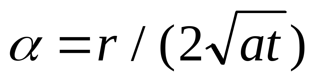 ,
,
t’ = t
= ,
и формула (3.3.1) принимает вид:
 .
.
(3.3.2)
Первый интеграл,
стоящий в скобках, известен из курса
высшей математики:
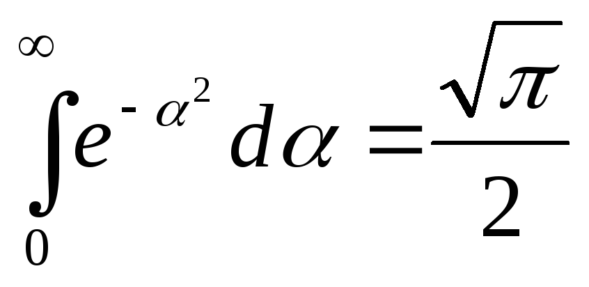
(интеграл
Пуассона),
а второй интеграл
через элементарные функции не выражается
и определяет специальную функцию,
которая называется функцией
ошибок Гаусса,
или интегралом
вероятностей,
или функцией эрфектум:
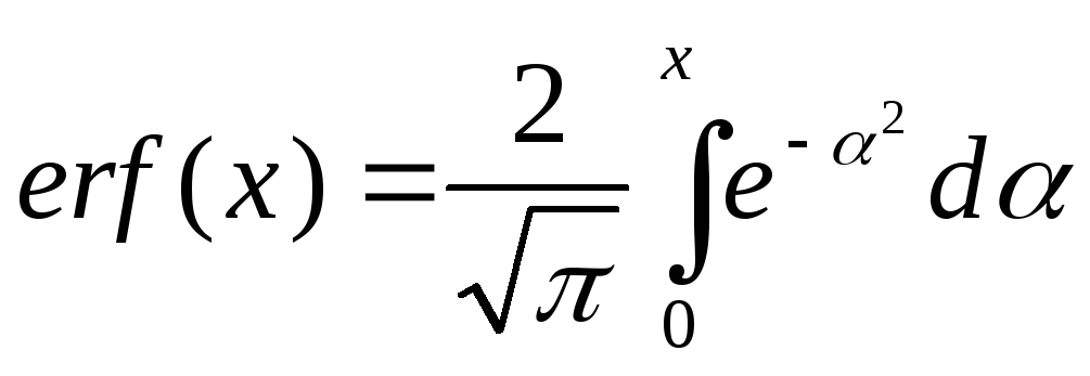
(3.3.3)
(читается «эрфектум»
или сокращенно: «эрф»). Через эту
функцию выражаются решения многих
задач в теории теплопроводности, да и
в других областях физики она играет
важную роль.
Из определения
(3.3.3) видно, что erf(0)
= 0, а erf()
= 1, т.е. erf(x)
— это монотонно возрастающая
функция, вид которой изображен
на Рис.3.3. Функция erf(x)
табулирована, и ее значения
приводятся в различных
справочниках; в таблице 3.1 приведены
несколько значений этой функции. В
библиотеках некоторых
языков программирования имеются
готовые подпрограммы для
вычисления функции erf(x).
Если готовой подпрограммы
нет, функцию erf(x)
можно
вычислить с помощью степенного
ряда. «Стандартное»
разложение этой функции в
степенной ряд, которое обычно
приводится в математических
справочниках, имеет вид:
 .
.
(3.3.4)
Э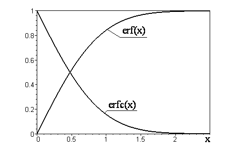 тот
тот
ряд удобен для анализа свойств функции,
но для практических расчетов он неудобен,
т.к. является знакопеременным, что
при вычислениях приводит к потере
точности. Более удобен следующий
ряд:
 ,
,
(3.3.5)
где
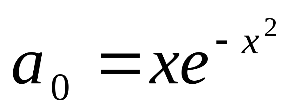 ,
,
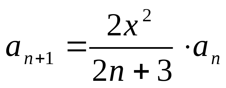 .
.
С
Рис. 3.3.
помощью этого ряда легко составить
программу вычисления erf(x)
на любом языке программирования
и даже на программируемом
микрокалькуляторе. Суммирование
надо прекращать, когда при
добавлении очередного an-го
слагаемого сумма перестанет меняться
(будет достигнута «машинная
точность»).
Если большой
точности не требуется, то можно
использовать приближенную формулу:
erf(x)
[1 — exp(-4x2/)]1/2.
(3.3.6)
Формула (3.3.6) дает
значения, абсолютная погрешность которых
не более 6.310-3,
а относительная погрешность
не более 0.71%.
Иногда требуется
определить erf(x)
в области отрицательных значений x.
Из формулы (3.3.3) очевидно, что erf(-x)
= — erf(x).
Заметим, что хотя
функция erf(x)
не является «элементарной», с точки
зрения ее свойств и способов
вычисления она проще, чем многие
«элементарные» функции, например,
тригонометрические.
С функцией erf(x)
связано еще несколько функций, часто
встречающихся в теплофизических
задачах. Это прежде всего дополнительный
интеграл вероятностей:
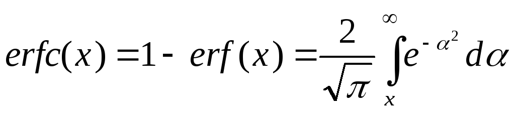 ,
,
(3.3.7)
который встречается
настолько часто, что для него используется
специальное обозначение: erfc(x)
(сокращенно читается «эрфик»). Вид
этой функции также приведен на рис.3.3.
Довольно часто
функцию erf(x)
приходится дифференцировать и
интегрировать. Из определения
(3.3.3) следует, что
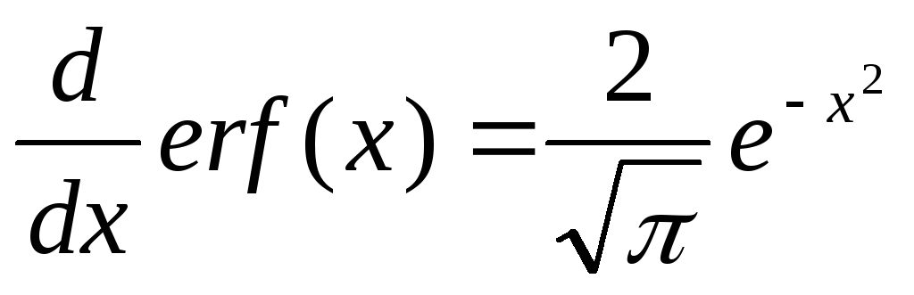 ,
,
(3.3.8)
а интеграл от
erfc(x)
(обозначается как ierfc(x))
равен:
 .
.
(3.3.9)
Вернемся к формуле
(3.3.2). Замечая, что ca
= ,
запишем эту формулу в виде:
 .
.
(3.3.10)
При t
значение функции
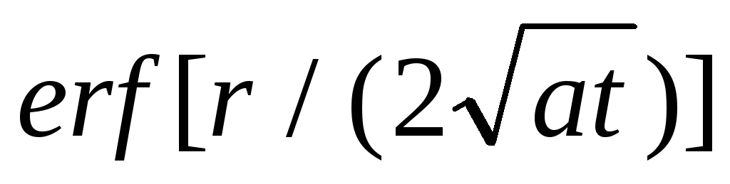
0,
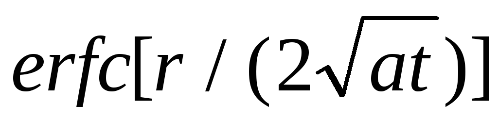
1, и формула (3.3.10), как и должно быть,
совпадает с формулой для
стационарного решения (если T0
принять за начало отсчета
температуры), т.к. при t
достигается стационарное
распределение температуры
в безграничной среде.
Таблица 3.1.
Некоторые значения функции erf(x).
|
x |
erf(x) |
x |
erf(x) |
x |
erf(x) |
x |
erf(x) |
x |
erf(x) |
|
0.0 |
0.0 |
0.3 |
0.32863 |
0.6 |
0.60386 |
0.9 |
0.79691 |
2.0 |
0.99532 |
|
0.1 |
0.11246 |
0.4 |
0.42839 |
0.7 |
0.67780 |
1.0 |
0.84270 |
2.5 |
0.99959 |
|
0.2 |
0.22270 |
0.5 |
0.52050 |
0.8 |
0.74210 |
1.5 |
0.96611 |
Соседние файлы в папке КраткийКонспектЛекций
- #
- #
- #
- #
- #
- #
- #
- #
- #
- #
- #
эрф | Функции ошибок, использующие cmath в C ++
В математике функция ошибки (также называемая функцией ошибки Гаусса) является специальной (неэлементарной) функцией сигмоидальной формы, которая встречается в уравнениях вероятности, статистики и дифференциальных уравнений в частных производных, описывающих диффузию.
Это вероятность того, что нормальная случайная величина со средним значением 0 и дисперсией 0,5 принимает значение между [-x, x]. Обозначается через erf (x) и рассчитывается как:

В cmath библиотеке C ++ функция ошибок уже была реализована. Есть две такие функции:
- erf (x) : эта встроенная функция вычисляет функцию ошибки для входного значения x. Параметр x, который может быть int или float или double. Возвращает двойное число, которое есть erf (x).
- erfc (x) : эта встроенная функция вычисляет дополнительную функцию ошибки для входного значения x. Параметр x, который может быть int или float или double. Возвращает двойное число, равное 1 — erf (x).
/ * C ++ код для использования erf * /
#include <iostream>
#include <cmath> /* erf */
Функция ошибки
В математике , то функция ошибок (также называется гауссовская ошибка функция ) является функция целого числа используется в анализе . Эта функция обозначается erf и является частью специальных функций . Это определяется:
Функция erf регулярно вмешивается в области вероятностей и статистики , а также в проблемы диффузии ( тепла или вещества ).
Резюме
Интерес этой функции
Вероятность и статистика
Вероятность того, что приведенная центрированная нормальная переменная X принимает значение в интервале [- z , z ], равна:
Функция распределения по X , или функция распределения нормального закона , как правило , обозначаются Ф, связана с функцией ошибки, ERF , обозначенное соотношением:
Проблемы диффузии
Функция ошибок участвует в выражении решений уравнения теплопроводности или уравнения диффузии , например, когда начальные условия задаются функцией Хевисайда .
Рассмотрим, в частности, полупространство x ≥ 0, занятое твердым телом с температуропроводностью κ и изначально однородной температурой T 1 . Если в момент времени t = 0 его граница x = 0 доведена до температуры T 2 , температура T ( x , t ) в любой момент времени t> 0 и в любой точке x > 0 определяется выражением:
Численный расчет
Интеграл не может быть получен с помощью замкнутой формулы, а путем разложения в целочисленный ряд (бесконечного радиуса сходимости), интегрированного по члену,
Существуют таблицы, в которых значения интегралов представлены в зависимости от z , но сегодня большинство числовых программ ( электронные таблицы , Scilab ) или CAS (например, Maple или MuPAD ) включают в себя процедуру вычисления erf (x) и ее взаимное смещение, инвертирование (x), которое еще более полезен при вычислении вероятностей .
Однако могут быть полезны следующие приближения:
- In (с погрешностью менее 6 × 10 –4 при x <0,5) v ( 0 ) , Эрф ( Икс ) знак равно 2 π е — Икс 2 ( Икс + 2 3 Икс 3 + 4 15 Икс 5 ) + о ( Икс 6 е — Икс 2 ) (x) = >> e ^ > left (x + > , x ^ + > , x ^ right) + o (x ^ , e ^ >)>
- In (с погрешностью менее 2 × 10 –4 при x > 1,75) v ( + ∞ ) , Эрф ( Икс ) знак равно 1 — е — Икс 2 1 π . ( 1 Икс — 1 2 Икс 3 + 3 4 Икс 5 — 15 8 Икс 7 ) + о ( Икс — 8 е — Икс 2 ) (x) = 1-e ^ >>>. left ( > — >> + >> — >> right) + o (x ^ e ^ >)>
- Для Икс > 0 , 1 — е — Икс 2 ≤ Эрф ( Икс ) ≤ 1 — е — 4 Икс 2 / π >>> leq operatorname (x) leq / pi>>>>
(схема, предложенная Дж. Т. Чу, 1955; верхняя граница приближается к функции erf всюду в пределах 7 × 10 −3 ).
- Для Икс > 0 , Эрф ( Икс ) ≃ 1 — е — 1 , 9 Икс 1 , 3 (x) simeq 1-e ^ >>
(приближение, предложенное Э. Робертом, 1996; оно приближается к функции erf везде в пределах 2,2 × 10 −2 . Приближение улучшается до менее 10 −2 для ). Икс ≥ 1
- Функция является решением дифференциального уравнения, имеющего значение 0 в 0 и производную в 0. Икс ↦ Эрф ( Икс ) × е Икс 2 (x) times e ^ >> y ″ — 2 Икс y ′ — 2 y знак равно 0 2 π >>>
Расширения
Бывает, что более общая функция определяется: E нет >
используется, а E 2 называется интегральной ошибкой.
Другие функции ошибок, используемые в анализе, в том числе:
- Дополнительная функция ошибок отметила ERFC и определяется по формуле:
- Функция ierfc (напротив) интеграла дополнительной функции ошибок erfc :
- Функция мнимой ошибки, отмеченная erfi , определяется следующим образом:
Часто он определяется только в некоторых программах компьютерной алгебры, таких как Mathematica и Maple . Тем не менее, его можно описать с помощью разложения в целочисленный ряд :
Взаимная функция

Функция обратной ошибки иногда используется в статистических формулах . Это можно описать с помощью последовательного расширения:
где и против 0 знак равно 1 = 1>
Получаем следующую разработку:
( радиус сходимости этого ряда равен 1, он дает хорошие приблизительные значения, например, только для | z | <1/2).
Документация
erf( x ) возвращает Функцию ошибок, оцененную для каждого элемента x .
Примеры
Нахождение функции ошибок
Найдите функцию ошибок значения.
Найдите функцию ошибок элементов вектора.
Найдите функцию ошибок элементов матрицы.
Нахождение кумулятивной функции распределения нормального распределения
Кумулятивная функция распределения (CDF) нормального, или Гауссова, распределения со стандартным отклонением σ и среднее значение μ
ϕ ( x ) = 1 2 ( 1 + e r f ( x — μ σ 2 ) ) .
Обратите внимание на то, что для увеличенной вычислительной точности, можно переписать формулу в терминах erfc . Для получения дополнительной информации смотрите Советы.
Постройте CDF нормального распределения с μ = 0 и σ = 1 .

Вычисление решения уравнения тепла с начальным условием
Где u ( x , t ) представляет температуру в положении x и время t , уравнение тепла
∂ u ∂ t = c ∂ 2 u ∂ x 2 ,
где c константа.
Для материала с коэффициентом тепла k , и для начального условия u ( x , 0 ) = a для x > b и u ( x , 0 ) = 0 в другом месте решение уравнения тепла
u ( x , t ) = a 2 ( e r f ( x — b 4 k t ) ) .
Для k = 2 , a = 5 , и b = 1 , постройте решение уравнения тепла во времена t = 0.1 , 5 , и 100 .

Входные параметры
x входной параметр
вещественное число | вектор из вещественных чисел | матрица вещественных чисел | многомерный массив вещественных чисел
Введите в виде вещественного числа, или вектора, матрицы или многомерного массива вещественных чисел. x не может быть разреженным.
Типы данных: single | double
Больше о
Функция ошибок
Функция ошибок erf x
erf( x )= 2 π ∫ 0 x e − t 2 d t .
Советы
Можно также найти стандартное нормальное распределение вероятностей с помощью функции normcdf (Statistics and Machine Learning Toolbox) . Отношение между функцией ошибок erf и normcdf
normcdf ( x ) = 1 2 ( 1 − erf ( − x 2 ) ) .
Для выражений формы 1 — erf(x) , используйте дополнительную функцию ошибок erfc вместо этого. Эта замена обеспечивает точность. Когда erf(x) близко к 1 , затем 1 — erf(x) небольшое число и может быть округлено в меньшую сторону до 0 . Вместо этого замена 1 — erf(x) с erfc(x) .
Расширенные возможности
«Высокие» массивы
Осуществление вычислений с массивами, которые содержат больше строк, чем помещается в памяти.
Генерация кода C/C++
Генерация кода C и C++ с помощью MATLAB® Coder™.
Указания и ограничения по применению:
Строгие вычисления с одинарной точностью не поддерживаются. В сгенерированном коде входные параметры с одинарной точностью производят выходные параметры с одинарной точностью. Однако переменные в функциональной силе быть с двойной точностью.
Основанная на потоке среда
Запустите код в фоновом режиме с помощью MATLAB® backgroundPool или ускорьте код с Parallel Computing Toolbox™ ThreadPool .
Эта функция полностью поддерживает основанные на потоке среды. Для получения дополнительной информации смотрите функции MATLAB Запуска в Основанной на потоке Среде.
Массивы графического процессора
Ускорьте код путем работы графического процессора (GPU) с помощью Parallel Computing Toolbox™.
Эта функция полностью поддерживает массивы графического процессора. Для получения дополнительной информации смотрите функции MATLAB Запуска на графическом процессоре (Parallel Computing Toolbox) .
Распределенные массивы
Большие массивы раздела через объединенную память о вашем кластере с помощью Parallel Computing Toolbox™.
Эта функция полностью поддерживает распределенные массивы. Для получения дополнительной информации смотрите функции MATLAB Запуска с Распределенными Массивами (Parallel Computing Toolbox) .
Смотрите также
Открытый пример
У вас есть модифицированная версия этого примера. Вы хотите открыть этот пример со своими редактированиями?
Документация MATLAB
Поддержка
© 1994-2021 The MathWorks, Inc.
1. Если смысл перевода понятен, то лучше оставьте как есть и не придирайтесь к словам, синонимам и тому подобному. О вкусах не спорим.
2. Не дополняйте перевод комментариями “от себя”. В исправлении не должно появляться дополнительных смыслов и комментариев, отсутствующих в оригинале. Такие правки не получится интегрировать в алгоритме автоматического перевода.
3. Сохраняйте структуру оригинального текста — например, не разбивайте одно предложение на два.
4. Не имеет смысла однотипное исправление перевода какого-то термина во всех предложениях. Исправляйте только в одном месте. Когда Вашу правку одобрят, это исправление будет алгоритмически распространено и на другие части документации.
5. По иным вопросам, например если надо исправить заблокированное для перевода слово, обратитесь к редакторам через форму технической поддержки.
Макеты страниц
7.3.1. Определение.
Функция вероятности ошибок  определяется-интегралом

Рассмотрим функцию Гаусса

Она изображается кривой, представленной на рис. 7.9. Площадь, заключенная между кривой  и осью абсцисс, равна единице. Действительно.
полагая  имеем
имеем

Согласно формуле (3) из п. 7.4.1, получаем

что и требовалось доказать.
Площадь между кривой  и осью абсцисс слева от абсциссы х обозначается через
  Следовательно,

Обе функции  играют большую роль в теории вероятности. Первая из них часто используется при анализе возмущений, распространяющихся по линиям передачи. Полезно установить зависимость между функциями
  так как функция
  подробно затабулирована Если положить
  то
то

Так как

то


Рис. 7.9.
7.3.2. Разложение функции Ф(x) в степенной ряд.
Достаточно проинтегрировать разложение в ряд  от нуля до х, чтобы получить степенной ряд

сходящийся при любом 
7.3.3. Разложение в асимптотический ряд функции 1 — Ф(x)
Имеем

Положим 

Повторно интегрируя  частям, получаем

Отсюда

Отношение абсолютных величин двух последовательных членов равно  Оно близко к единице, если
  близко к
  Ясно, что член асимптотического разложения
  соответствующий этому
  имеет наименьшую абсолютную величину. Именно на нем и следует остановиться, чтобы получить наименьшую ошибку при вычислении
Замечание. В примере 3 п. 2.2.8 мы показали, что функция Гаусса  представленная на рис. 7.9, обладает свойством быть своей собственной трансформантой Фурье. Поэтому понятна та важная роль, которую она играет при изучении спектра сигналов и диаграмм направленности источников радиоволн.
7.3.4. Выражение функции 1 — Ф(x/2) через интеграл Коши.
В разложении функции  в степенной ряд заменим х на
  Получаем

Согласно результатам п. 7.4.3, имеем ( целое)

Это дает возможность написать

Согласно формуле (10) п. 7.4.5. (см. также рис. 7.12),

Отсюда

и

Функция  удовлетворяет условиям леммы Жордана
Поэтому мы можем также написать

7.3.5. Таблица функции …
(см. скан)
7.3.6. График функции …

Рис. 7.10.
1. Нормальное распределение (распределение Гаусса)
Если случайная величина $ X $ подчиняется распределению вероятностей с позиционным параметром $ mu $ и параметром масштаба $ sigma $, а ее функция плотности вероятности равна
$$ f(x) = frac{1}{sqrt{2pi},sigma} e^{-frac{(x-mu)^2}{2 {sigma} ^2}} $$
Тогда эта случайная величина называется нормальной случайной величиной, а распределение, которому подчиняется нормальная случайная величина, называется нормальным распределением и обозначается как $ X Thicksim N ( mu, sigma ^ 2) $.
Когда $ mu = 0, sigma = 1 $, это называется стандартным нормальным распределением. $ X Thicksim N (0, 1) $
$$ f(x) = frac{1}{sqrt{2pi}} e^{-frac{x^2}{2 }} $$
На следующем рисунке показано общее нормальное распределение.

На следующем рисунке показано стандартное общее распределение.

Функция распределения общего нормального распределения $ F (x) $
$$F(x)=P(X leqslant x)= frac{1}{sqrt{2pi} sigma}int_{-infty}^{x}e^{-tfrac{(t-mu)^2}{2{sigma}^2}}dt $$
Функция распределения стандартного нормального распределения $ Phi (x) $:
$$Phi(x)=P(X leqslant x) = frac{1}{sqrt{2pi} }int_{-infty}^{x}e^{-tfrac{t^2}{2}}dt $$


2.Q функция
Функция Q также называется функцией правого хвоста стандартного нормального распределения.
$$Q(x)=int_x^inftyfrac{1}{sqrt{2pi}} e^{-tfrac{t^2}{2}}dt = 1-Phi(x) $$

3. Функция ошибки
$$ erf(x)=frac{2}{sqrt{ pi}}int_0^{x}e^{-t^2}dt $$
4. Дополнительная функция ошибок
$$ erfc(x)=frac{2}{sqrt{ pi}}int_x^{infty}e^{-t^2}dt = 1-erf(x) $$

5. Отношения между ними
$$ Q(x) = 1-Phi(x) $$
$$ Q(x) = frac{1}{2} erfc(x/ sqrt 2) $$
$$ erfc(x) = 2Q(sqrt 2 x) $$
$$ erf(x) = 1-2Q(sqrt 2 x) $$
$$ erf(x) + erfc(x) = 1 $$
Заметка:
Поскольку полный интеграл функции плотности нормального распределения равен 1 (то есть вероятность P (X <∞) = 1):

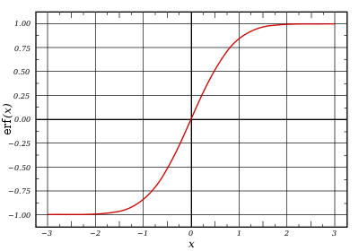

График функции ошибок
В математике функция ошибок (функция Лапласа) — это неэлементарная функция, возникающая в теории вероятностей, статистике и теории дифференциальных уравнений в частных производных. Она определяется как
 .
.
Дополнительная функция ошибок, обозначаемая  (иногда применяется обозначение
  ) определяется через функцию ошибок:
 .
.
Комплексная функция ошибок, обозначаемая  , также определяется через функцию ошибок:
 .
.
Содержание
- 1 Свойства
- 2 Применение
- 3 Асимптотическое разложение
- 4 Родственные функции
- 4.1 Обобщённые функции ошибок
- 4.2 Итерированные интегралы дополнительной функции ошибок
- 5 Реализация
- 6 См. также
- 7 Литература
- 8 Ссылки
Свойства
- Функция ошибок нечётна:

- Для любого комплексного
 выполняется

где черта обозначает комплексное сопряжение числа .
- Функция ошибок не может быть представлена через элементарные функции, но, разлагая интегрируемое выражение в ряд Тейлора и интегрируя почленно, мы можем получить её представление в виде ряда:

Это равенство выполняется (и ряд сходится) как для любого вещественного [источник не указан 302 дня], так и на всей комплексной плоскости. Последовательность знаменателей образует последовательность A007680 в OEIS.
- Для итеративного вычисления элементов ряда полезно представить его в альтернативном виде:

поскольку  — сомножитель, превращающий
  -й член ряда в
  -й, считая первым членом .
- Функция ошибок на бесконечности равна единице; однако это справедливо только при приближении к бесконечности по вещественной оси, так как:
- При рассмотрении функции ошибок в комплексной плоскости точка
 будет для неё существенно особой.
- Производная функции ошибок выводится непосредственно из определения функции:

- Обратная функция ошибок представляет собой ряд

где c0 = 1 и

Поэтому ряд можно представить в следующем виде (заметим, что дроби сокращены):
 [1]
[1]
Последовательности числителей и знаменателей после сокращения — A092676 и A132467 в OEIS; последовательность числителей до сокращения — A002067 в OEIS.

Дополнительная функция ошибок
Применение
Если набор случайных чисел подчиняется нормальному распределению со стандартным отклонением  , то вероятность, что число отклонится от среднего не более чем на
  , равна
  .
.
Функция ошибок и дополнительная функция ошибок встречаются в решении некоторых дифференциальных уравнений, например, уравнения теплопроводности с граничными условиями описываемыми функцией Хевисайда («ступенькой»).
В системах цифровой оптической коммуникации, вероятность ошибки на бит также выражается формулой, использующей функцию ошибок.
Асимптотическое разложение
При больших полезно асимптотическое разложение для дополнительной функции ошибок:
![operatorname{erfc},x = frac{e^{-x^2}}{xsqrt{pi}}left [1+sum_{n=1}^infty (-1)^n frac{1cdot3cdot5cdots(2n-1)}{(2x^2)^n}right ]=frac{e^{-x^2}}{xsqrt{pi}}sum_{n=0}^infty (-1)^n frac{(2n)!}{n!(2x)^{2n}}.,](https://dic.academic.ru/dic.nsf/ruwiki/32769b5d42152b6b316dfca7a42e23eb.png)
Хотя для любого конечного этот ряд расходится, на практике первых нескольких членов достаточно для вычисления с хорошей точностью, в то время как ряд Тейлора сходится очень медленно.
Другое приближение даётся формулой

где

Родственные функции
С точностью до масштаба и сдвига, функция ошибок совпадает с нормальным интегральным распределением, обозначаемым 

Обратная функция к  , известная как нормальная квантильная функция, иногда обозначается
  и выражается через нормальную функцию ошибок как

Нормальное интегральное распределение чаще применяется в теории вероятностей и математической статистике, в то время как функция ошибок чаще применяется в других разделах математики.
Функция ошибок является частным случаем функции Миттаг-Леффлера, а также может быть представлена как вырожденная гипергеометрическая функция (функция Куммера):

Функция ошибок выражается также через интеграл Френеля. В терминах регуляризованной неполной гамма-функции P и неполной гамма-функции,

Обобщённые функции ошибок
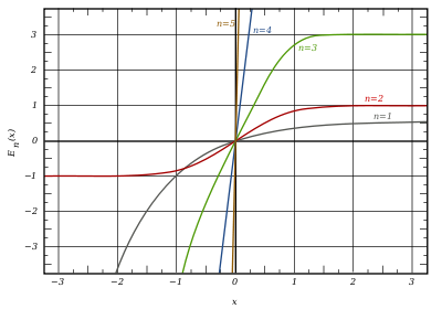
Некоторые авторы обсуждают более общие функции

Примечательными частными случаями являются:
После деления на  все
все  с нечётными
  выглядят похоже (но не идентично). Все с чётными тоже выглядят похоже, но не идентично, после деления на . Все обобщённые функции ошибок с
  выглядят похоже на полуоси
  .
.
На полуоси все обобщённые функции могут быть выражены через гамма-функцию:

Следовательно, мы можем выразить функцию ошибок через гамма-функцию:

Итерированные интегралы дополнительной функции ошибок
Итерированные интегралы дополнительной функции ошибок определяются как

Их можно разложить в ряд:

откуда следуют свойства симметрии

и

Реализация
В стандарте языка Си (ISO/IEC 9899:1999, 7.12.8) предусмотрены функция ошибок  и дополнительная функция ошибок
  . Функции находятся в заголовочных файлах
 math.h или cmath. Там же есть пары функций erff(),erfcf() и erfl(),erfcl(). Первая пара получает и возвращает значения типа float, а вторая — значения типа long double. Соответствующие функции также содержатся в библиотеке Math проекта Boost.
В языке Java функции ошибок нет в стандартной библиотеке математических функций java.lang.Math [2]. Класс Erf есть в пакете org.apache.commons.math.special от Apache [3]. Однако эта библиотека не является одной из стандартных библиотек Java 6.
Matlab[4], Mathematica и Maxima[5] содержат обычную и дополнительную функцию ошибок, а также обратные к ним функции.
В языке Python функция ошибок доступна из стандартной библиотеки math, начиная с версии 2.7. [6] Также функция ошибок, дополнительная функция ошибок и многие другие специальные функции определены в модуле Special проекта SciPy [7].
В языке Erlang функция ошибок и дополнительная функция ошибок доступны из стандартного модуля math, [8].
См. также
- Функция Гаусса
- Функция Доусона
Литература
- Milton Abramowitz and Irene A. Stegun, eds. Handbook of Mathematical Functions with Formulas, Graphs, and Mathematical Tables. New York: Dover, 1972. (См. часть 7)
- Nikolai G. Lehtinen «Error functions», April 2010 [9]
Ссылки
- MathWorld — Erf
- Онлайновый калькулятор Erf и много других специальных функций (до 6 знаков)
- Онлайновый калькулятор, вычисляющий в том числе Erf