4.3. Метод коррекции ошибок FEC (Forward Error Correction)
Транспортировка данных подвержена влиянию шумов и наводок, которые вносят искажения. Если вероятность повреждения данных мала, достаточно зарегистрировать сам факт искажения и повторить передачу поврежденного фрагмента.
Когда вероятность искажения велика, например, в каналах коммуникаций с геостационарными спутниками, используются методы коррекции ошибок. Одним из таких методов является FEC (Forward Error Correction, иногда называемое канальным кодированием ) [4.1]. Технология FEC в последнее время достаточно широко используется в беспроводных локальных сетях (WLAN). Существуют две основные разновидности FEC: блочное кодирование и кодирование по методу свертки.
Блочное кодирование работает с блоками (пакетами) бит или символов фиксированного размера. Метод свертки работает с потоками бит или символов произвольной протяженности. Коды свертки при желании могут быть преобразованы в блочные коды.
Существует большое число блочных кодов, одним из наиболее важных является алгоритм Рида-Соломона, который используется при работе с CD, DVD и жесткими дисками ЭВМ. Блочные коды и коды свертки могут использоваться и совместно.
Для FEC -кодирования иногда используется метод сверки, который впервые был применен в 1955 году. Главной особенностью этого метода является сильная зависимость кодирования от предыдущих информационных битов и высокие требования к объему памяти. FEC -код обычно просматривает при декодировании 2-8 бит десятки или даже сотни бит, полученных ранее.
В 1967 году Эндрю Витерби (Andrew Viterbi) разработал технику декодирования, которая стала стандартной для кодов свертки. Эта методика требовала меньше памяти. Метод свертки более эффективен, когда ошибки распределены случайным образом, а не группируются в кластеры. Работа же с кластерами ошибок более эффективна при использовании алгебраического кодирования.
Одной из широко применяемых разновидностей коррекции ошибок является турбо-кодирование, разработанное американской аэрокосмической корпорацией. В этой схеме комбинируется два или более относительно простых кодов свертки. В FEC, так же как и в других методах коррекции ошибок (коды Хэмминга, алгоритм Рида-Соломона и др.), блоки данных из k бит снабжаются кодами четности, которые пересылаются вместе с данными и обеспечивают не только детектирование, но и исправление ошибок. Каждый дополнительный (избыточный) бит является сложной функцией многих исходных информационных бит. Исходная информация может содержаться в выходном передаваемом коде, тогда такой код называется систематическим, а может и не содержаться.
В результате через канал передается n -битовое кодовое слово ( n>k ). Конкретная реализация алгоритма FEC характеризуется комбинацией ( n, k ). Применение FEC в Интернете регламентируется документом RFC3452. Коды FEC могут исключить необходимость обратной связи при потере или искажении доставленных данных (запросы повторной передачи). Особенно привлекательна технология FEC при работе с мультикастинг-потоками, где ретрансмиссия не предусматривается (см. RFC-3453).
В 1974 году Йозеф Оденвальдер (Joseph odenwalder) объединил возможности алгебраического кодирования и метода свертки. Хорошего результата можно добиться, введя специальную операцию псевдослучайного перемешивания бит (interleaver).
В 1993 году группой Клода Берроу (Claude Berrou) был разработан турбо-код. В кодеке, реализующем этот алгоритм, содержатся кодировщики как минимум двух компонент (реализующие алгебраический метод или свертку). Кодирование осуществляется для блоков данных. Здесь также используется псевдослучайное перемешивание бит перед передачей. Это приводит к тому, что кластеры ошибок, внесенных при транспортировке, оказываются разнесенными случайным образом в пределах блока данных.
На
рис.
4.8 проводится сравнение вариантов BER (Bit Error Rate) при обычной транспортировке данных через канал и при передаче тех же данных с использованием коррекции ошибок FEC для разных значений отношения сигнал-шум ( S/N ). Из этих данных видно, что при отношении S/N= 8 дБ применение FEC позволяет понизить BER примерно в 100 раз. При этом достигается результат, близкий (в пределах одного децибела) к теоретическому пределу Шеннона.
За последние пять лет были разработаны программы, которые позволяют оптимизировать структуры турбо-кодов. Улучшение BER для турбокодов имеет асимптотический предел, и дальнейшее увеличение S/N уже не дает никакого выигрыша. Но схемы, позволяющие смягчить влияние этого насыщения, продолжают разрабатываться.
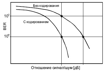
Рис.
4.8.
Турбо-кодек должен иметь столько же компонентных декодеров, сколько имеется кодировщиков на стороне передатчика. Декодеры соединяются последовательно.
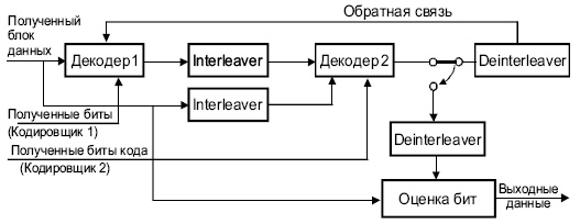
Рис.
4.9.
Турбо-декодер
Техника FEC находит все большее применение в телекоммуникациях, например, при передачи мультимедиа [2].
Следует помнить, что, как в случае FEC , так и в других известных методах коррекции ошибок ( BCH , Golay, Hamming и др.) скорректированный код является верным лишь с определенной конечной вероятностью.
 Прямая коррекция ошибок (FEC) это метод, который использовался в течении нескольких лет в подводных оптоволоконных системах, проложенных по морскому дну. Этот метод позволяет с почти идеальной точностью передать данные, даже если передача осуществляется по каналу с большим количеством шумов. В настоящее время используется несколько алгоритмов FEC, таких как код Хэмминга, кода Рида-Соломона и код БЧХ.
В качестве примера, рассмотрим работу вашего мобильного телефона в условиях слабого сигнала сотовой сети. Допустим, вы хотели сказать человеку на другом конце линии некую последовательность чисел. Есть несколько методов, которые можно использовать для повышения точности. Предположим, что список чисел, которые вы хотите передать, это 7, 3, 8, 10, 12 и 21. Одним из способов может быть повтор списка чисел два раза. Запишите каждый список и сравните их, если они совпадают, передача данных, вероятно, корректна. Основным недостатком такого метода является то, что, поскольку данные передаются дважды, пропускная способность системы делится пополам и, если списки не совпадают, у вас не будет ни малейшего представления, который из них верный. Используя этот метод, для того, чтобы убедиться в хорошем качестве передачи и исправить некоторые ошибки, вам придется отправить данные три раза и проверить, что два из трех списков полностью совпадают. Второй способ будет выглядеть примерно так: в первую очередь, вы будете отправлять количество чисел, которые необходимо принять, затем саму последовательно, и в конце последует передача числа, являющегося суммой последовательности. Передаваемое сообщение при этом примет следующий вид: 6, 7, 3, 8, 10, 12, 21, и 67. Человек, принимающий сообщение, будет смотреть на первое число, чтобы затем убедится, что будет получено правильное количество чисел в сообщении, а затем проверит, что число в конце последовательности, действительно является суммой переданных чисел. Этот метод требует отправки значительно меньшего количества дополнительных данных. Если любое полученное число неверно или пропущено, то число контрольной суммы в конце передачи не будет соответствовать сумме, передаваемых чисел. Показанные выше методы представляют собой примеры кода обнаружения ошибок. Они позволяют определить, была ли передача точной, но не позволяют исправлять ошибки.
Примечание: Термин «Forward» в аббревиатуре FEC означает, что исправление ошибок осуществляется путем передачи некоторой информации вместе с передачей данных.
Код исправления ошибок считаются более сложными, в сравнении с кодом обнаружения ошибок и используются почти в каждом современном коммуникационном приложении. Также, коды исправления ошибок нашли широкое применение в CD и DVD проигрывателях. Для того, чтобы привести пример кода исправления ошибок, нужно ввести и объяснить два термина: двоичность и чётность. В предыдущих примерах кода обнаружения ошибок, мы использовали такие числа, как 7, 3, 8, и т.д. Это базовые числа системы исчисления, знакомой нам в повседневной жизни. Двоичные числа в основе имеют два числа, которые могут иметь только два возможных значения – 0 или 1. Бинарная система используется почти во всех коммуникационных и компьютерных системах. Второе определение, которое необходимо разобрать, называется четность. Чётность — термин, который используется в двоичных системах связи, чтобы указать, является ли число единиц в передаче четным или же нет. Если число единиц является четным, то чётность совпадает и наоборот.
Код Хэмминга
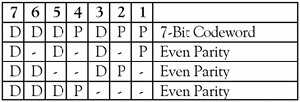
Рассмотрим сообщение, имеющее четыре бита данных (D), которое должно быть передано в 7-битной кодировке с добавлением трёх битов данных для поиска и устранения ошибок. Этот код будет называться (7, 4). Это означает, что общая длина кода составляет семь битов, но только четыре из них на самом деле данные. Три добавленных бита — это три бита проверки на четность (Р), где чётность каждого вычисляется в разных группах битов сообщения, как показано на рисунке 1.
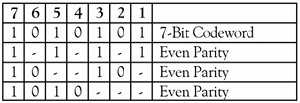
Например, сообщение 1011 будут направлено, как 1010101, как показано на рисунке 2.
Можно заметить, что в случае возникновения ошибки в любом из семи битов, эта ошибка оказывает влияние на различные комбинации трех битов четности в зависимости от битовой позиции.
Например, предположим, что вышеупомянутое сообщение 1010101 передаётся и возникает один бит ошибки, так что получено кодовое слово 1110101:
Передача Приём
Сообщение Сообщение
1 0 1 0 1 0 1 ————> 1 1 1 0 1 0 1
Эта ошибка может быть исправлена путем определения, какой из трех битов четности пострадал, как показано на рисунке ниже:
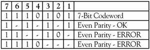
Характер ошибок четности битов указывает, какой бит в кодовом слове с ошибкой, таким образом, он может быть исправлен.
Основные функции кода Хэмминга можно резюмировать:
- Обнаружение 2-битовых ошибок (при условии отсутствия ошибок корректировка не выполняется)
- Коррекция единичных ошибочных битов
- 3 проверочных бита добавляется к 4-битовому сообщению
Способность корректировать одиночные ошибочные биты приводит к снижению себестоимости передачи, которая получается меньше, чем в случае отправки сообщения дважды целиком. (Напомним, что, просто отправив сообщение дважды коррекция ошибок не выполняется.) К тому же, при увеличении размера кодового слова, дополнительная нагрузка исправления ошибочных битов уменьшается. Например, одним из возможных вариантов кода Хэмминга для передачи по морским подводным оптоволоконным системам является код (18880, 18865). Это означает, что кодовое слово 18880 в действительности содержит 18,865 бит данных и 15 бит коррекции ошибок. Более надежные методы прямой коррекции ошибок (FEC) могут содержать гораздо больше битов коррекции ошибок, так что несколько ошибочных битов могут быть обнаружены и исправлены в каждом кодовом слове.
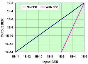 Существует метод прямой коррекции ошибок (FEC), аналогичный коду Хемминга. Как правило, в системах с оптической несущей ОС-192, накладывается около 7% дополнительной нагрузки на систему за счёт процесса коррекции ошибок (FEC). Допустим, базовая скорость передачи данных 10 Гбит/с, с учётом дополнительной нагрузки будет увеличена до 10,7 Гбит/с. Таким образом, с каждой 1000 бит передаваемых данных, отправляется ещё 70 бит коррекции ошибок, чтобы позволить провести проверку целостности полученных данных и исправить ошибки, которые могут возникнуть при передаче по оптическому каналу связи. На рисунке 4 показано влияние прямой коррекции (FEC) на системный коэффициент ошибочных битов (BER). Этот коэффициент является показателем числа ошибок в битах, деленное на общее число переданных битов в исследуемом временном интервале. BER 10-3 означает, что один из каждых 1000 бит будет передан некорректно. Синий график наглядно отображает количество передаваемых данных, если система не имеет FEC. Входной коэффициент BER (input BER) – это показатель ошибок, возникающих в канале передачи. Пока в системе отсутствует FEC, любые ошибки, которые происходят во время передачи появляются на выходе системы. Фиолетовый график показывает, что может произойти, если в системе используется FEC. В отсутствии FEC в системе входной коэффициент BER 10-6 даст аналогичное значение выходного BER 10-6, а в случае использования данной технологии происходит значительное улучшение выходной величины BER 10-14 (output BER).
Таким образом, интеграция прямой коррекции ошибок в систему позволяет разработчику увеличивать расстояние и скорости передачи данных значительнее, чем при использовании любой другой технологии, а также увеличит срок службы системы.
«Interleaver» redirects here. For the fiber-optic device, see optical interleaver.
In computing, telecommunication, information theory, and coding theory, an error correction code, sometimes error correcting code, (ECC) is used for controlling errors in data over unreliable or noisy communication channels.[1][2] The central idea is the sender encodes the message with redundant information in the form of an ECC. The redundancy allows the receiver to detect a limited number of errors that may occur anywhere in the message, and often to correct these errors without retransmission. The American mathematician Richard Hamming pioneered this field in the 1940s and invented the first error-correcting code in 1950: the Hamming (7,4) code.[2]
ECC contrasts with error detection in that errors that are encountered can be corrected, not simply detected. The advantage is that a system using ECC does not require a reverse channel to request retransmission of data when an error occurs. The downside is that there is a fixed overhead that is added to the message, thereby requiring a higher forward-channel bandwidth. ECC is therefore applied in situations where retransmissions are costly or impossible, such as one-way communication links and when transmitting to multiple receivers in multicast. Long-latency connections also benefit; in the case of a satellite orbiting around Uranus, retransmission due to errors can create a delay of five hours. ECC information is usually added to mass storage devices to enable recovery of corrupted data, is widely used in modems, and is used on systems where the primary memory is ECC memory.
ECC processing in a receiver may be applied to a digital bitstream or in the demodulation of a digitally modulated carrier. For the latter, ECC is an integral part of the initial analog-to-digital conversion in the receiver. The Viterbi decoder implements a soft-decision algorithm to demodulate digital data from an analog signal corrupted by noise. Many ECC encoders/decoders can also generate a bit-error rate (BER) signal, which can be used as feedback to fine-tune the analog receiving electronics.
The maximum fractions of errors or of missing bits that can be corrected are determined by the design of the ECC code, so different error correcting codes are suitable for different conditions. In general, a stronger code induces more redundancy that needs to be transmitted using the available bandwidth, which reduces the effective bit-rate while improving the received effective signal-to-noise ratio. The noisy-channel coding theorem of Claude Shannon can be used to compute the maximum achievable communication bandwidth for a given maximum acceptable error probability. This establishes bounds on the theoretical maximum information transfer rate of a channel with some given base noise level. However, the proof is not constructive, and hence gives no insight of how to build a capacity achieving code. After years of research, some advanced ECC systems as of 2016[3] come very close to the theoretical maximum.
Forward error correction[edit]
In telecommunication, information theory, and coding theory, forward error correction (FEC) or channel coding[4][3] is a technique used for controlling errors in data transmission over unreliable or noisy communication channels. The central idea is that the sender encodes the message in a redundant way, most often by using an ECC.
The redundancy allows the receiver to detect a limited number of errors that may occur anywhere in the message, and often to correct these errors without re-transmission. FEC gives the receiver the ability to correct errors without needing a reverse channel to request re-transmission of data, but at the cost of a fixed, higher forward channel bandwidth. FEC is therefore applied in situations where re-transmissions are costly or impossible, such as one-way communication links and when transmitting to multiple receivers in multicast. FEC information is usually added to mass storage (magnetic, optical and solid state/flash based) devices to enable recovery of corrupted data, is widely used in modems, is used on systems where the primary memory is ECC memory and in broadcast situations, where the receiver does not have capabilities to request re-transmission or doing so would induce significant latency. For example, in the case of a satellite orbiting Uranus, a re-transmission because of decoding errors would create a delay of at least 5 hours.
FEC processing in a receiver may be applied to a digital bit stream or in the demodulation of a digitally modulated carrier. For the latter, FEC is an integral part of the initial analog-to-digital conversion in the receiver. The Viterbi decoder implements a soft-decision algorithm to demodulate digital data from an analog signal corrupted by noise. Many FEC coders can also generate a bit-error rate (BER) signal which can be used as feedback to fine-tune the analog receiving electronics.
The maximum proportion of errors or missing bits that can be corrected is determined by the design of the ECC, so different forward error correcting codes are suitable for different conditions. In general, a stronger code induces more redundancy that needs to be transmitted using the available bandwidth, which reduces the effective bit-rate while improving the received effective signal-to-noise ratio. The noisy-channel coding theorem of Claude Shannon answers the question of how much bandwidth is left for data communication while using the most efficient code that turns the decoding error probability to zero. This establishes bounds on the theoretical maximum information transfer rate of a channel with some given base noise level. His proof is not constructive, and hence gives no insight of how to build a capacity achieving code. However, after years of research, some advanced FEC systems like polar code[3] achieve the Shannon channel capacity under the hypothesis of an infinite length frame.
How it works[edit]
ECC is accomplished by adding redundancy to the transmitted information using an algorithm. A redundant bit may be a complex function of many original information bits. The original information may or may not appear literally in the encoded output; codes that include the unmodified input in the output are systematic, while those that do not are non-systematic.
A simplistic example of ECC is to transmit each data bit 3 times, which is known as a (3,1) repetition code. Through a noisy channel, a receiver might see 8 versions of the output, see table below.
| Triplet received | Interpreted as |
|---|---|
| 000 | 0 (error-free) |
| 001 | 0 |
| 010 | 0 |
| 100 | 0 |
| 111 | 1 (error-free) |
| 110 | 1 |
| 101 | 1 |
| 011 | 1 |
This allows an error in any one of the three samples to be corrected by «majority vote», or «democratic voting». The correcting ability of this ECC is:
- Up to 1 bit of triplet in error, or
- up to 2 bits of triplet omitted (cases not shown in table).
Though simple to implement and widely used, this triple modular redundancy is a relatively inefficient ECC. Better ECC codes typically examine the last several tens or even the last several hundreds of previously received bits to determine how to decode the current small handful of bits (typically in groups of 2 to 8 bits).
Averaging noise to reduce errors[edit]
ECC could be said to work by «averaging noise»; since each data bit affects many transmitted symbols, the corruption of some symbols by noise usually allows the original user data to be extracted from the other, uncorrupted received symbols that also depend on the same user data.
- Because of this «risk-pooling» effect, digital communication systems that use ECC tend to work well above a certain minimum signal-to-noise ratio and not at all below it.
- This all-or-nothing tendency – the cliff effect – becomes more pronounced as stronger codes are used that more closely approach the theoretical Shannon limit.
- Interleaving ECC coded data can reduce the all or nothing properties of transmitted ECC codes when the channel errors tend to occur in bursts. However, this method has limits; it is best used on narrowband data.
Most telecommunication systems use a fixed channel code designed to tolerate the expected worst-case bit error rate, and then fail to work at all if the bit error rate is ever worse.
However, some systems adapt to the given channel error conditions: some instances of hybrid automatic repeat-request use a fixed ECC method as long as the ECC can handle the error rate, then switch to ARQ when the error rate gets too high;
adaptive modulation and coding uses a variety of ECC rates, adding more error-correction bits per packet when there are higher error rates in the channel, or taking them out when they are not needed.
Types of ECC[edit]

A block code (specifically a Hamming code) where redundant bits are added as a block to the end of the initial message
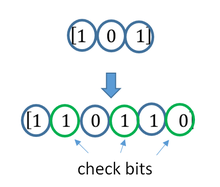
A continuous code convolutional code where redundant bits are added continuously into the structure of the code word
The two main categories of ECC codes are block codes and convolutional codes.
- Block codes work on fixed-size blocks (packets) of bits or symbols of predetermined size. Practical block codes can generally be hard-decoded in polynomial time to their block length.
- Convolutional codes work on bit or symbol streams of arbitrary length. They are most often soft decoded with the Viterbi algorithm, though other algorithms are sometimes used. Viterbi decoding allows asymptotically optimal decoding efficiency with increasing constraint length of the convolutional code, but at the expense of exponentially increasing complexity. A convolutional code that is terminated is also a ‘block code’ in that it encodes a block of input data, but the block size of a convolutional code is generally arbitrary, while block codes have a fixed size dictated by their algebraic characteristics. Types of termination for convolutional codes include «tail-biting» and «bit-flushing».
There are many types of block codes; Reed–Solomon coding is noteworthy for its widespread use in compact discs, DVDs, and hard disk drives. Other examples of classical block codes include Golay, BCH, Multidimensional parity, and Hamming codes.
Hamming ECC is commonly used to correct NAND flash memory errors.[5]
This provides single-bit error correction and 2-bit error detection.
Hamming codes are only suitable for more reliable single-level cell (SLC) NAND.
Denser multi-level cell (MLC) NAND may use multi-bit correcting ECC such as BCH or Reed–Solomon.[6][7] NOR Flash typically does not use any error correction.[6]
Classical block codes are usually decoded using hard-decision algorithms,[8] which means that for every input and output signal a hard decision is made whether it corresponds to a one or a zero bit. In contrast, convolutional codes are typically decoded using soft-decision algorithms like the Viterbi, MAP or BCJR algorithms, which process (discretized) analog signals, and which allow for much higher error-correction performance than hard-decision decoding.
Nearly all classical block codes apply the algebraic properties of finite fields. Hence classical block codes are often referred to as algebraic codes.
In contrast to classical block codes that often specify an error-detecting or error-correcting ability, many modern block codes such as LDPC codes lack such guarantees. Instead, modern codes are evaluated in terms of their bit error rates.
Most forward error correction codes correct only bit-flips, but not bit-insertions or bit-deletions.
In this setting, the Hamming distance is the appropriate way to measure the bit error rate.
A few forward error correction codes are designed to correct bit-insertions and bit-deletions, such as Marker Codes and Watermark Codes.
The Levenshtein distance is a more appropriate way to measure the bit error rate when using such codes.
[9]
Code-rate and the tradeoff between reliability and data rate[edit]
The fundamental principle of ECC is to add redundant bits in order to help the decoder to find out the true message that was encoded by the transmitter. The code-rate of a given ECC system is defined as the ratio between the number of information bits and the total number of bits (i.e., information plus redundancy bits) in a given communication package. The code-rate is hence a real number. A low code-rate close to zero implies a strong code that uses many redundant bits to achieve a good performance, while a large code-rate close to 1 implies a weak code.
The redundant bits that protect the information have to be transferred using the same communication resources that they are trying to protect. This causes a fundamental tradeoff between reliability and data rate.[10] In one extreme, a strong code (with low code-rate) can induce an important increase in the receiver SNR (signal-to-noise-ratio) decreasing the bit error rate, at the cost of reducing the effective data rate. On the other extreme, not using any ECC (i.e., a code-rate equal to 1) uses the full channel for information transfer purposes, at the cost of leaving the bits without any additional protection.
One interesting question is the following: how efficient in terms of information transfer can an ECC be that has a negligible decoding error rate? This question was answered by Claude Shannon with his second theorem, which says that the channel capacity is the maximum bit rate achievable by any ECC whose error rate tends to zero:[11] His proof relies on Gaussian random coding, which is not suitable to real-world applications. The upper bound given by Shannon’s work inspired a long journey in designing ECCs that can come close to the ultimate performance boundary. Various codes today can attain almost the Shannon limit. However, capacity achieving ECCs are usually extremely complex to implement.
The most popular ECCs have a trade-off between performance and computational complexity. Usually, their parameters give a range of possible code rates, which can be optimized depending on the scenario. Usually, this optimization is done in order to achieve a low decoding error probability while minimizing the impact to the data rate. Another criterion for optimizing the code rate is to balance low error rate and retransmissions number in order to the energy cost of the communication.[12]
Concatenated ECC codes for improved performance[edit]
Classical (algebraic) block codes and convolutional codes are frequently combined in concatenated coding schemes in which a short constraint-length Viterbi-decoded convolutional code does most of the work and a block code (usually Reed–Solomon) with larger symbol size and block length «mops up» any errors made by the convolutional decoder. Single pass decoding with this family of error correction codes can yield very low error rates, but for long range transmission conditions (like deep space) iterative decoding is recommended.
Concatenated codes have been standard practice in satellite and deep space communications since Voyager 2 first used the technique in its 1986 encounter with Uranus. The Galileo craft used iterative concatenated codes to compensate for the very high error rate conditions caused by having a failed antenna.
Low-density parity-check (LDPC)[edit]
Low-density parity-check (LDPC) codes are a class of highly efficient linear block
codes made from many single parity check (SPC) codes. They can provide performance very close to the channel capacity (the theoretical maximum) using an iterated soft-decision decoding approach, at linear time complexity in terms of their block length. Practical implementations rely heavily on decoding the constituent SPC codes in parallel.
LDPC codes were first introduced by Robert G. Gallager in his PhD thesis in 1960,
but due to the computational effort in implementing encoder and decoder and the introduction of Reed–Solomon codes,
they were mostly ignored until the 1990s.
LDPC codes are now used in many recent high-speed communication standards, such as DVB-S2 (Digital Video Broadcasting – Satellite – Second Generation), WiMAX (IEEE 802.16e standard for microwave communications), High-Speed Wireless LAN (IEEE 802.11n),[13] 10GBase-T Ethernet (802.3an) and G.hn/G.9960 (ITU-T Standard for networking over power lines, phone lines and coaxial cable). Other LDPC codes are standardized for wireless communication standards within 3GPP MBMS (see fountain codes).
Turbo codes[edit]
Turbo coding is an iterated soft-decoding scheme that combines two or more relatively simple convolutional codes and an interleaver to produce a block code that can perform to within a fraction of a decibel of the Shannon limit. Predating LDPC codes in terms of practical application, they now provide similar performance.
One of the earliest commercial applications of turbo coding was the CDMA2000 1x (TIA IS-2000) digital cellular technology developed by Qualcomm and sold by Verizon Wireless, Sprint, and other carriers. It is also used for the evolution of CDMA2000 1x specifically for Internet access, 1xEV-DO (TIA IS-856). Like 1x, EV-DO was developed by Qualcomm, and is sold by Verizon Wireless, Sprint, and other carriers (Verizon’s marketing name for 1xEV-DO is Broadband Access, Sprint’s consumer and business marketing names for 1xEV-DO are Power Vision and Mobile Broadband, respectively).
Local decoding and testing of codes[edit]
Sometimes it is only necessary to decode single bits of the message, or to check whether a given signal is a codeword, and do so without looking at the entire signal. This can make sense in a streaming setting, where codewords are too large to be classically decoded fast enough and where only a few bits of the message are of interest for now. Also such codes have become an important tool in computational complexity theory, e.g., for the design of probabilistically checkable proofs.
Locally decodable codes are error-correcting codes for which single bits of the message can be probabilistically recovered by only looking at a small (say constant) number of positions of a codeword, even after the codeword has been corrupted at some constant fraction of positions. Locally testable codes are error-correcting codes for which it can be checked probabilistically whether a signal is close to a codeword by only looking at a small number of positions of the signal.
Interleaving[edit]
«Interleaver» redirects here. For the fiber-optic device, see optical interleaver.

A short illustration of interleaving idea
Interleaving is frequently used in digital communication and storage systems to improve the performance of forward error correcting codes. Many communication channels are not memoryless: errors typically occur in bursts rather than independently. If the number of errors within a code word exceeds the error-correcting code’s capability, it fails to recover the original code word. Interleaving alleviates this problem by shuffling source symbols across several code words, thereby creating a more uniform distribution of errors.[14] Therefore, interleaving is widely used for burst error-correction.
The analysis of modern iterated codes, like turbo codes and LDPC codes, typically assumes an independent distribution of errors.[15] Systems using LDPC codes therefore typically employ additional interleaving across the symbols within a code word.[16]
For turbo codes, an interleaver is an integral component and its proper design is crucial for good performance.[14][17] The iterative decoding algorithm works best when there are not short cycles in the factor graph that represents the decoder; the interleaver is chosen to avoid short cycles.
Interleaver designs include:
- rectangular (or uniform) interleavers (similar to the method using skip factors described above)
- convolutional interleavers
- random interleavers (where the interleaver is a known random permutation)
- S-random interleaver (where the interleaver is a known random permutation with the constraint that no input symbols within distance S appear within a distance of S in the output).[18]
- a contention-free quadratic permutation polynomial (QPP).[19] An example of use is in the 3GPP Long Term Evolution mobile telecommunication standard.[20]
In multi-carrier communication systems, interleaving across carriers may be employed to provide frequency diversity, e.g., to mitigate frequency-selective fading or narrowband interference.[21]
Example[edit]
Transmission without interleaving:
Error-free message:                                 aaaabbbbccccddddeeeeffffgggg
Transmission with a burst error:                    aaaabbbbccc____deeeeffffgggg
Here, each group of the same letter represents a 4-bit one-bit error-correcting codeword. The codeword cccc is altered in one bit and can be corrected, but the codeword dddd is altered in three bits, so either it cannot be decoded at all or it might be decoded incorrectly.
With interleaving:
Error-free code words:                              aaaabbbbccccddddeeeeffffgggg
Interleaved:                                        abcdefgabcdefgabcdefgabcdefg
Transmission with a burst error:                    abcdefgabcd____bcdefgabcdefg
Received code words after deinterleaving:           aa_abbbbccccdddde_eef_ffg_gg
In each of the codewords «aaaa», «eeee», «ffff», and «gggg», only one bit is altered, so one-bit error-correcting code will decode everything correctly.
Transmission without interleaving:
Original transmitted sentence:                      ThisIsAnExampleOfInterleaving
Received sentence with a burst error:               ThisIs______pleOfInterleaving
The term «AnExample» ends up mostly unintelligible and difficult to correct.
With interleaving:
Transmitted sentence:                               ThisIsAnExampleOfInterleaving...
Error-free transmission:                            TIEpfeaghsxlIrv.iAaenli.snmOten.
Received sentence with a burst error:               TIEpfe______Irv.iAaenli.snmOten.
Received sentence after deinterleaving:             T_isI_AnE_amp_eOfInterle_vin_...
No word is completely lost and the missing letters can be recovered with minimal guesswork.
Disadvantages of interleaving[edit]
Use of interleaving techniques increases total delay. This is because the entire interleaved block must be received before the packets can be decoded.[22] Also interleavers hide the structure of errors; without an interleaver, more advanced decoding algorithms can take advantage of the error structure and achieve more reliable communication than a simpler decoder combined with an interleaver[citation needed]. An example of such an algorithm is based on neural network[23] structures.
Software for error-correcting codes[edit]
Simulating the behaviour of error-correcting codes (ECCs) in software is a common practice to design, validate and improve ECCs. The upcoming wireless 5G standard raises a new range of applications for the software ECCs: the Cloud Radio Access Networks (C-RAN) in a Software-defined radio (SDR) context. The idea is to directly use software ECCs in the communications. For instance in the 5G, the software ECCs could be located in the cloud and the antennas connected to this computing resources: improving this way the flexibility of the communication network and eventually increasing the energy efficiency of the system.
In this context, there are various available Open-source software listed below (non exhaustive).
- AFF3CT(A Fast Forward Error Correction Toolbox): a full communication chain in C++ (many supported codes like Turbo, LDPC, Polar codes, etc.), very fast and specialized on channel coding (can be used as a program for simulations or as a library for the SDR).
- IT++: a C++ library of classes and functions for linear algebra, numerical optimization, signal processing, communications, and statistics.
- OpenAir: implementation (in C) of the 3GPP specifications concerning the Evolved Packet Core Networks.
List of error-correcting codes[edit]
| Distance | Code |
|---|---|
| 2 (single-error detecting) | Parity |
| 3 (single-error correcting) | Triple modular redundancy |
| 3 (single-error correcting) | perfect Hamming such as Hamming(7,4) |
| 4 (SECDED) | Extended Hamming |
| 5 (double-error correcting) | |
| 6 (double-error correct-/triple error detect) | Nordstrom-Robinson code |
| 7 (three-error correcting) | perfect binary Golay code |
| 8 (TECFED) | extended binary Golay code |
- AN codes
- BCH code, which can be designed to correct any arbitrary number of errors per code block.
- Barker code used for radar, telemetry, ultra sound, Wifi, DSSS mobile phone networks, GPS etc.
- Berger code
- Constant-weight code
- Convolutional code
- Expander codes
- Group codes
- Golay codes, of which the Binary Golay code is of practical interest
- Goppa code, used in the McEliece cryptosystem
- Hadamard code
- Hagelbarger code
- Hamming code
- Latin square based code for non-white noise (prevalent for example in broadband over powerlines)
- Lexicographic code
- Linear Network Coding, a type of erasure correcting code across networks instead of point-to-point links
- Long code
- Low-density parity-check code, also known as Gallager code, as the archetype for sparse graph codes
- LT code, which is a near-optimal rateless erasure correcting code (Fountain code)
- m of n codes
- Nordstrom-Robinson code, used in Geometry and Group Theory[24]
- Online code, a near-optimal rateless erasure correcting code
- Polar code (coding theory)
- Raptor code, a near-optimal rateless erasure correcting code
- Reed–Solomon error correction
- Reed–Muller code
- Repeat-accumulate code
- Repetition codes, such as Triple modular redundancy
- Spinal code, a rateless, nonlinear code based on pseudo-random hash functions[25]
- Tornado code, a near-optimal erasure correcting code, and the precursor to Fountain codes
- Turbo code
- Walsh–Hadamard code
- Cyclic redundancy checks (CRCs) can correct 1-bit errors for messages at most
bits long for optimal generator polynomials of degree
, see Mathematics of cyclic redundancy checks#Bitfilters
See also[edit]
- Code rate
- Erasure codes
- Soft-decision decoder
- Burst error-correcting code
- Error detection and correction
- Error-correcting codes with feedback
References[edit]
- ^ Glover, Neal; Dudley, Trent (1990). Practical Error Correction Design For Engineers (Revision 1.1, 2nd ed.). CO, USA: Cirrus Logic. ISBN 0-927239-00-0.
- ^ a b Hamming, Richard Wesley (April 1950). «Error Detecting and Error Correcting Codes». Bell System Technical Journal. USA: AT&T. 29 (2): 147–160. doi:10.1002/j.1538-7305.1950.tb00463.x. S2CID 61141773.
- ^ a b c Maunder, Robert (2016). «Overview of Channel Coding».
- ^ Charles Wang; Dean Sklar; Diana Johnson (Winter 2001–2002). «Forward Error-Correction Coding». Crosslink. The Aerospace Corporation. 3 (1). Archived from the original on 14 March 2012. Retrieved 5 March 2006.
How Forward Error-Correcting Codes Work
- ^ «Hamming codes for NAND flash memory devices» Archived 21 August 2016 at the Wayback Machine. EE Times-Asia. Apparently based on «Micron Technical Note TN-29-08: Hamming Codes for NAND Flash Memory Devices». 2005. Both say: «The Hamming algorithm is an industry-accepted method for error detection and correction in many SLC NAND flash-based applications.»
- ^ a b «What Types of ECC Should Be Used on Flash Memory?» (Application note). Spansion. 2011.
Both Reed–Solomon algorithm and BCH algorithm are common ECC choices for MLC NAND flash. … Hamming based block codes are the most commonly used ECC for SLC…. both Reed–Solomon and BCH are able to handle multiple errors and are widely used on MLC flash.
- ^ Jim Cooke (August 2007). «The Inconvenient Truths of NAND Flash Memory» (PDF). p. 28.
For SLC, a code with a correction threshold of 1 is sufficient. t=4 required … for MLC.
- ^ Baldi, M.; Chiaraluce, F. (2008). «A Simple Scheme for Belief Propagation Decoding of BCH and RS Codes in Multimedia Transmissions». International Journal of Digital Multimedia Broadcasting. 2008: 1–12. doi:10.1155/2008/957846.
- ^ Shah, Gaurav; Molina, Andres; Blaze, Matt (2006). «Keyboards and covert channels». USENIX. Retrieved 20 December 2018.
- ^ Tse, David; Viswanath, Pramod (2005), Fundamentals of Wireless Communication, Cambridge University Press, UK
- ^ Shannon, C. E. (1948). «A mathematical theory of communication» (PDF). Bell System Technical Journal. 27 (3–4): 379–423 & 623–656. doi:10.1002/j.1538-7305.1948.tb01338.x. hdl:11858/00-001M-0000-002C-4314-2.
- ^ Rosas, F.; Brante, G.; Souza, R. D.; Oberli, C. (2014). «Optimizing the code rate for achieving energy-efficient wireless communications». Proceedings of the IEEE Wireless Communications and Networking Conference (WCNC). pp. 775–780. doi:10.1109/WCNC.2014.6952166. ISBN 978-1-4799-3083-8.
- ^ IEEE Standard, section 20.3.11.6 «802.11n-2009» Archived 3 February 2013 at the Wayback Machine, IEEE, 29 October 2009, accessed 21 March 2011.
- ^ a b Vucetic, B.; Yuan, J. (2000). Turbo codes: principles and applications. Springer Verlag. ISBN 978-0-7923-7868-6.
- ^ Luby, Michael; Mitzenmacher, M.; Shokrollahi, A.; Spielman, D.; Stemann, V. (1997). «Practical Loss-Resilient Codes». Proc. 29th Annual Association for Computing Machinery (ACM) Symposium on Theory of Computation.
- ^ «Digital Video Broadcast (DVB); Second generation framing structure, channel coding and modulation systems for Broadcasting, Interactive Services, News Gathering and other satellite broadband applications (DVB-S2)». En 302 307. ETSI (V1.2.1). April 2009.
- ^ Andrews, K. S.; Divsalar, D.; Dolinar, S.; Hamkins, J.; Jones, C. R.; Pollara, F. (November 2007). «The Development of Turbo and LDPC Codes for Deep-Space Applications». Proceedings of the IEEE. 95 (11): 2142–2156. doi:10.1109/JPROC.2007.905132. S2CID 9289140.
- ^ Dolinar, S.; Divsalar, D. (15 August 1995). «Weight Distributions for Turbo Codes Using Random and Nonrandom Permutations». TDA Progress Report. 122: 42–122. Bibcode:1995TDAPR.122…56D. CiteSeerX 10.1.1.105.6640.
- ^ Takeshita, Oscar (2006). «Permutation Polynomial Interleavers: An Algebraic-Geometric Perspective». IEEE Transactions on Information Theory. 53 (6): 2116–2132. arXiv:cs/0601048. Bibcode:2006cs……..1048T. doi:10.1109/TIT.2007.896870. S2CID 660.
- ^ 3GPP TS 36.212, version 8.8.0, page 14
- ^ «Digital Video Broadcast (DVB); Frame structure, channel coding and modulation for a second generation digital terrestrial television broadcasting system (DVB-T2)». En 302 755. ETSI (V1.1.1). September 2009.
- ^ Techie (3 June 2010). «Explaining Interleaving». W3 Techie Blog. Retrieved 3 June 2010.
- ^ Krastanov, Stefan; Jiang, Liang (8 September 2017). «Deep Neural Network Probabilistic Decoder for Stabilizer Codes». Scientific Reports. 7 (1): 11003. arXiv:1705.09334. Bibcode:2017NatSR…711003K. doi:10.1038/s41598-017-11266-1. PMC 5591216. PMID 28887480.
- ^ Nordstrom, A.W.; Robinson, J.P. (1967), «An optimum nonlinear code», Information and Control, 11 (5–6): 613–616, doi:10.1016/S0019-9958(67)90835-2
- ^ Perry, Jonathan; Balakrishnan, Hari; Shah, Devavrat (2011). «Rateless Spinal Codes». Proceedings of the 10th ACM Workshop on Hot Topics in Networks. pp. 1–6. doi:10.1145/2070562.2070568. hdl:1721.1/79676. ISBN 9781450310598.
Further reading[edit]
- MacWilliams, Florence Jessiem; Sloane, Neil James Alexander (2007) [1977]. Written at AT&T Shannon Labs, Florham Park, New Jersey, USA. The Theory of Error-Correcting Codes. North-Holland Mathematical Library. Vol. 16 (digital print of 12th impression, 1st ed.). Amsterdam / London / New York / Tokyo: North-Holland / Elsevier BV. ISBN 978-0-444-85193-2. LCCN 76-41296. (xxii+762+6 pages)
- Clark, Jr., George C.; Cain, J. Bibb (1981). Error-Correction Coding for Digital Communications. New York, USA: Plenum Press. ISBN 0-306-40615-2.
- Arazi, Benjamin (1987). Swetman, Herb (ed.). A Commonsense Approach to the Theory of Error Correcting Codes. MIT Press Series in Computer Systems. Vol. 10 (1 ed.). Cambridge, Massachusetts, USA / London, UK: Massachusetts Institute of Technology. ISBN 0-262-01098-4. LCCN 87-21889. (x+2+208+4 pages)
- Wicker, Stephen B. (1995). Error Control Systems for Digital Communication and Storage. Englewood Cliffs, New Jersey, USA: Prentice-Hall. ISBN 0-13-200809-2.
- Wilson, Stephen G. (1996). Digital Modulation and Coding. Englewood Cliffs, New Jersey, USA: Prentice-Hall. ISBN 0-13-210071-1.
- «Error Correction Code in Single Level Cell NAND Flash memories» 2007-02-16
- «Error Correction Code in NAND Flash memories» 2004-11-29
- Observations on Errors, Corrections, & Trust of Dependent Systems, by James Hamilton, 2012-02-26
- Sphere Packings, Lattices and Groups, By J. H. Conway, Neil James Alexander Sloane, Springer Science & Business Media, 2013-03-09 – Mathematics – 682 pages.
External links[edit]
- Morelos-Zaragoza, Robert (2004). «The Correcting Codes (ECC) Page». Retrieved 5 March 2006.
- lpdec: library for LP decoding and related things (Python)
«Interleaver» redirects here. For the fiber-optic device, see optical interleaver.
In computing, telecommunication, information theory, and coding theory, an error correction code, sometimes error correcting code, (ECC) is used for controlling errors in data over unreliable or noisy communication channels.[1][2] The central idea is the sender encodes the message with redundant information in the form of an ECC. The redundancy allows the receiver to detect a limited number of errors that may occur anywhere in the message, and often to correct these errors without retransmission. The American mathematician Richard Hamming pioneered this field in the 1940s and invented the first error-correcting code in 1950: the Hamming (7,4) code.[2]
ECC contrasts with error detection in that errors that are encountered can be corrected, not simply detected. The advantage is that a system using ECC does not require a reverse channel to request retransmission of data when an error occurs. The downside is that there is a fixed overhead that is added to the message, thereby requiring a higher forward-channel bandwidth. ECC is therefore applied in situations where retransmissions are costly or impossible, such as one-way communication links and when transmitting to multiple receivers in multicast. Long-latency connections also benefit; in the case of a satellite orbiting around Uranus, retransmission due to errors can create a delay of five hours. ECC information is usually added to mass storage devices to enable recovery of corrupted data, is widely used in modems, and is used on systems where the primary memory is ECC memory.
ECC processing in a receiver may be applied to a digital bitstream or in the demodulation of a digitally modulated carrier. For the latter, ECC is an integral part of the initial analog-to-digital conversion in the receiver. The Viterbi decoder implements a soft-decision algorithm to demodulate digital data from an analog signal corrupted by noise. Many ECC encoders/decoders can also generate a bit-error rate (BER) signal, which can be used as feedback to fine-tune the analog receiving electronics.
The maximum fractions of errors or of missing bits that can be corrected are determined by the design of the ECC code, so different error correcting codes are suitable for different conditions. In general, a stronger code induces more redundancy that needs to be transmitted using the available bandwidth, which reduces the effective bit-rate while improving the received effective signal-to-noise ratio. The noisy-channel coding theorem of Claude Shannon can be used to compute the maximum achievable communication bandwidth for a given maximum acceptable error probability. This establishes bounds on the theoretical maximum information transfer rate of a channel with some given base noise level. However, the proof is not constructive, and hence gives no insight of how to build a capacity achieving code. After years of research, some advanced ECC systems as of 2016[3] come very close to the theoretical maximum.
Forward error correction[edit]
In telecommunication, information theory, and coding theory, forward error correction (FEC) or channel coding[4][3] is a technique used for controlling errors in data transmission over unreliable or noisy communication channels. The central idea is that the sender encodes the message in a redundant way, most often by using an ECC.
The redundancy allows the receiver to detect a limited number of errors that may occur anywhere in the message, and often to correct these errors without re-transmission. FEC gives the receiver the ability to correct errors without needing a reverse channel to request re-transmission of data, but at the cost of a fixed, higher forward channel bandwidth. FEC is therefore applied in situations where re-transmissions are costly or impossible, such as one-way communication links and when transmitting to multiple receivers in multicast. FEC information is usually added to mass storage (magnetic, optical and solid state/flash based) devices to enable recovery of corrupted data, is widely used in modems, is used on systems where the primary memory is ECC memory and in broadcast situations, where the receiver does not have capabilities to request re-transmission or doing so would induce significant latency. For example, in the case of a satellite orbiting Uranus, a re-transmission because of decoding errors would create a delay of at least 5 hours.
FEC processing in a receiver may be applied to a digital bit stream or in the demodulation of a digitally modulated carrier. For the latter, FEC is an integral part of the initial analog-to-digital conversion in the receiver. The Viterbi decoder implements a soft-decision algorithm to demodulate digital data from an analog signal corrupted by noise. Many FEC coders can also generate a bit-error rate (BER) signal which can be used as feedback to fine-tune the analog receiving electronics.
The maximum proportion of errors or missing bits that can be corrected is determined by the design of the ECC, so different forward error correcting codes are suitable for different conditions. In general, a stronger code induces more redundancy that needs to be transmitted using the available bandwidth, which reduces the effective bit-rate while improving the received effective signal-to-noise ratio. The noisy-channel coding theorem of Claude Shannon answers the question of how much bandwidth is left for data communication while using the most efficient code that turns the decoding error probability to zero. This establishes bounds on the theoretical maximum information transfer rate of a channel with some given base noise level. His proof is not constructive, and hence gives no insight of how to build a capacity achieving code. However, after years of research, some advanced FEC systems like polar code[3] achieve the Shannon channel capacity under the hypothesis of an infinite length frame.
How it works[edit]
ECC is accomplished by adding redundancy to the transmitted information using an algorithm. A redundant bit may be a complex function of many original information bits. The original information may or may not appear literally in the encoded output; codes that include the unmodified input in the output are systematic, while those that do not are non-systematic.
A simplistic example of ECC is to transmit each data bit 3 times, which is known as a (3,1) repetition code. Through a noisy channel, a receiver might see 8 versions of the output, see table below.
| Triplet received | Interpreted as |
|---|---|
| 000 | 0 (error-free) |
| 001 | 0 |
| 010 | 0 |
| 100 | 0 |
| 111 | 1 (error-free) |
| 110 | 1 |
| 101 | 1 |
| 011 | 1 |
This allows an error in any one of the three samples to be corrected by «majority vote», or «democratic voting». The correcting ability of this ECC is:
- Up to 1 bit of triplet in error, or
- up to 2 bits of triplet omitted (cases not shown in table).
Though simple to implement and widely used, this triple modular redundancy is a relatively inefficient ECC. Better ECC codes typically examine the last several tens or even the last several hundreds of previously received bits to determine how to decode the current small handful of bits (typically in groups of 2 to 8 bits).
Averaging noise to reduce errors[edit]
ECC could be said to work by «averaging noise»; since each data bit affects many transmitted symbols, the corruption of some symbols by noise usually allows the original user data to be extracted from the other, uncorrupted received symbols that also depend on the same user data.
- Because of this «risk-pooling» effect, digital communication systems that use ECC tend to work well above a certain minimum signal-to-noise ratio and not at all below it.
- This all-or-nothing tendency – the cliff effect – becomes more pronounced as stronger codes are used that more closely approach the theoretical Shannon limit.
- Interleaving ECC coded data can reduce the all or nothing properties of transmitted ECC codes when the channel errors tend to occur in bursts. However, this method has limits; it is best used on narrowband data.
Most telecommunication systems use a fixed channel code designed to tolerate the expected worst-case bit error rate, and then fail to work at all if the bit error rate is ever worse.
However, some systems adapt to the given channel error conditions: some instances of hybrid automatic repeat-request use a fixed ECC method as long as the ECC can handle the error rate, then switch to ARQ when the error rate gets too high;
adaptive modulation and coding uses a variety of ECC rates, adding more error-correction bits per packet when there are higher error rates in the channel, or taking them out when they are not needed.
Types of ECC[edit]
A block code (specifically a Hamming code) where redundant bits are added as a block to the end of the initial message
A continuous code convolutional code where redundant bits are added continuously into the structure of the code word
The two main categories of ECC codes are block codes and convolutional codes.
- Block codes work on fixed-size blocks (packets) of bits or symbols of predetermined size. Practical block codes can generally be hard-decoded in polynomial time to their block length.
- Convolutional codes work on bit or symbol streams of arbitrary length. They are most often soft decoded with the Viterbi algorithm, though other algorithms are sometimes used. Viterbi decoding allows asymptotically optimal decoding efficiency with increasing constraint length of the convolutional code, but at the expense of exponentially increasing complexity. A convolutional code that is terminated is also a ‘block code’ in that it encodes a block of input data, but the block size of a convolutional code is generally arbitrary, while block codes have a fixed size dictated by their algebraic characteristics. Types of termination for convolutional codes include «tail-biting» and «bit-flushing».
There are many types of block codes; Reed–Solomon coding is noteworthy for its widespread use in compact discs, DVDs, and hard disk drives. Other examples of classical block codes include Golay, BCH, Multidimensional parity, and Hamming codes.
Hamming ECC is commonly used to correct NAND flash memory errors.[5]
This provides single-bit error correction and 2-bit error detection.
Hamming codes are only suitable for more reliable single-level cell (SLC) NAND.
Denser multi-level cell (MLC) NAND may use multi-bit correcting ECC such as BCH or Reed–Solomon.[6][7] NOR Flash typically does not use any error correction.[6]
Classical block codes are usually decoded using hard-decision algorithms,[8] which means that for every input and output signal a hard decision is made whether it corresponds to a one or a zero bit. In contrast, convolutional codes are typically decoded using soft-decision algorithms like the Viterbi, MAP or BCJR algorithms, which process (discretized) analog signals, and which allow for much higher error-correction performance than hard-decision decoding.
Nearly all classical block codes apply the algebraic properties of finite fields. Hence classical block codes are often referred to as algebraic codes.
In contrast to classical block codes that often specify an error-detecting or error-correcting ability, many modern block codes such as LDPC codes lack such guarantees. Instead, modern codes are evaluated in terms of their bit error rates.
Most forward error correction codes correct only bit-flips, but not bit-insertions or bit-deletions.
In this setting, the Hamming distance is the appropriate way to measure the bit error rate.
A few forward error correction codes are designed to correct bit-insertions and bit-deletions, such as Marker Codes and Watermark Codes.
The Levenshtein distance is a more appropriate way to measure the bit error rate when using such codes.
[9]
Code-rate and the tradeoff between reliability and data rate[edit]
The fundamental principle of ECC is to add redundant bits in order to help the decoder to find out the true message that was encoded by the transmitter. The code-rate of a given ECC system is defined as the ratio between the number of information bits and the total number of bits (i.e., information plus redundancy bits) in a given communication package. The code-rate is hence a real number. A low code-rate close to zero implies a strong code that uses many redundant bits to achieve a good performance, while a large code-rate close to 1 implies a weak code.
The redundant bits that protect the information have to be transferred using the same communication resources that they are trying to protect. This causes a fundamental tradeoff between reliability and data rate.[10] In one extreme, a strong code (with low code-rate) can induce an important increase in the receiver SNR (signal-to-noise-ratio) decreasing the bit error rate, at the cost of reducing the effective data rate. On the other extreme, not using any ECC (i.e., a code-rate equal to 1) uses the full channel for information transfer purposes, at the cost of leaving the bits without any additional protection.
One interesting question is the following: how efficient in terms of information transfer can an ECC be that has a negligible decoding error rate? This question was answered by Claude Shannon with his second theorem, which says that the channel capacity is the maximum bit rate achievable by any ECC whose error rate tends to zero:[11] His proof relies on Gaussian random coding, which is not suitable to real-world applications. The upper bound given by Shannon’s work inspired a long journey in designing ECCs that can come close to the ultimate performance boundary. Various codes today can attain almost the Shannon limit. However, capacity achieving ECCs are usually extremely complex to implement.
The most popular ECCs have a trade-off between performance and computational complexity. Usually, their parameters give a range of possible code rates, which can be optimized depending on the scenario. Usually, this optimization is done in order to achieve a low decoding error probability while minimizing the impact to the data rate. Another criterion for optimizing the code rate is to balance low error rate and retransmissions number in order to the energy cost of the communication.[12]
Concatenated ECC codes for improved performance[edit]
Classical (algebraic) block codes and convolutional codes are frequently combined in concatenated coding schemes in which a short constraint-length Viterbi-decoded convolutional code does most of the work and a block code (usually Reed–Solomon) with larger symbol size and block length «mops up» any errors made by the convolutional decoder. Single pass decoding with this family of error correction codes can yield very low error rates, but for long range transmission conditions (like deep space) iterative decoding is recommended.
Concatenated codes have been standard practice in satellite and deep space communications since Voyager 2 first used the technique in its 1986 encounter with Uranus. The Galileo craft used iterative concatenated codes to compensate for the very high error rate conditions caused by having a failed antenna.
Low-density parity-check (LDPC)[edit]
Low-density parity-check (LDPC) codes are a class of highly efficient linear block
codes made from many single parity check (SPC) codes. They can provide performance very close to the channel capacity (the theoretical maximum) using an iterated soft-decision decoding approach, at linear time complexity in terms of their block length. Practical implementations rely heavily on decoding the constituent SPC codes in parallel.
LDPC codes were first introduced by Robert G. Gallager in his PhD thesis in 1960,
but due to the computational effort in implementing encoder and decoder and the introduction of Reed–Solomon codes,
they were mostly ignored until the 1990s.
LDPC codes are now used in many recent high-speed communication standards, such as DVB-S2 (Digital Video Broadcasting – Satellite – Second Generation), WiMAX (IEEE 802.16e standard for microwave communications), High-Speed Wireless LAN (IEEE 802.11n),[13] 10GBase-T Ethernet (802.3an) and G.hn/G.9960 (ITU-T Standard for networking over power lines, phone lines and coaxial cable). Other LDPC codes are standardized for wireless communication standards within 3GPP MBMS (see fountain codes).
Turbo codes[edit]
Turbo coding is an iterated soft-decoding scheme that combines two or more relatively simple convolutional codes and an interleaver to produce a block code that can perform to within a fraction of a decibel of the Shannon limit. Predating LDPC codes in terms of practical application, they now provide similar performance.
One of the earliest commercial applications of turbo coding was the CDMA2000 1x (TIA IS-2000) digital cellular technology developed by Qualcomm and sold by Verizon Wireless, Sprint, and other carriers. It is also used for the evolution of CDMA2000 1x specifically for Internet access, 1xEV-DO (TIA IS-856). Like 1x, EV-DO was developed by Qualcomm, and is sold by Verizon Wireless, Sprint, and other carriers (Verizon’s marketing name for 1xEV-DO is Broadband Access, Sprint’s consumer and business marketing names for 1xEV-DO are Power Vision and Mobile Broadband, respectively).
Local decoding and testing of codes[edit]
Sometimes it is only necessary to decode single bits of the message, or to check whether a given signal is a codeword, and do so without looking at the entire signal. This can make sense in a streaming setting, where codewords are too large to be classically decoded fast enough and where only a few bits of the message are of interest for now. Also such codes have become an important tool in computational complexity theory, e.g., for the design of probabilistically checkable proofs.
Locally decodable codes are error-correcting codes for which single bits of the message can be probabilistically recovered by only looking at a small (say constant) number of positions of a codeword, even after the codeword has been corrupted at some constant fraction of positions. Locally testable codes are error-correcting codes for which it can be checked probabilistically whether a signal is close to a codeword by only looking at a small number of positions of the signal.
Interleaving[edit]
«Interleaver» redirects here. For the fiber-optic device, see optical interleaver.
A short illustration of interleaving idea
Interleaving is frequently used in digital communication and storage systems to improve the performance of forward error correcting codes. Many communication channels are not memoryless: errors typically occur in bursts rather than independently. If the number of errors within a code word exceeds the error-correcting code’s capability, it fails to recover the original code word. Interleaving alleviates this problem by shuffling source symbols across several code words, thereby creating a more uniform distribution of errors.[14] Therefore, interleaving is widely used for burst error-correction.
The analysis of modern iterated codes, like turbo codes and LDPC codes, typically assumes an independent distribution of errors.[15] Systems using LDPC codes therefore typically employ additional interleaving across the symbols within a code word.[16]
For turbo codes, an interleaver is an integral component and its proper design is crucial for good performance.[14][17] The iterative decoding algorithm works best when there are not short cycles in the factor graph that represents the decoder; the interleaver is chosen to avoid short cycles.
Interleaver designs include:
- rectangular (or uniform) interleavers (similar to the method using skip factors described above)
- convolutional interleavers
- random interleavers (where the interleaver is a known random permutation)
- S-random interleaver (where the interleaver is a known random permutation with the constraint that no input symbols within distance S appear within a distance of S in the output).[18]
- a contention-free quadratic permutation polynomial (QPP).[19] An example of use is in the 3GPP Long Term Evolution mobile telecommunication standard.[20]
In multi-carrier communication systems, interleaving across carriers may be employed to provide frequency diversity, e.g., to mitigate frequency-selective fading or narrowband interference.[21]
Example[edit]
Transmission without interleaving:
Error-free message:                                 aaaabbbbccccddddeeeeffffgggg
Transmission with a burst error:                    aaaabbbbccc____deeeeffffgggg
Here, each group of the same letter represents a 4-bit one-bit error-correcting codeword. The codeword cccc is altered in one bit and can be corrected, but the codeword dddd is altered in three bits, so either it cannot be decoded at all or it might be decoded incorrectly.
With interleaving:
Error-free code words:                              aaaabbbbccccddddeeeeffffgggg
Interleaved:                                        abcdefgabcdefgabcdefgabcdefg
Transmission with a burst error:                    abcdefgabcd____bcdefgabcdefg
Received code words after deinterleaving:           aa_abbbbccccdddde_eef_ffg_gg
In each of the codewords «aaaa», «eeee», «ffff», and «gggg», only one bit is altered, so one-bit error-correcting code will decode everything correctly.
Transmission without interleaving:
Original transmitted sentence:                      ThisIsAnExampleOfInterleaving
Received sentence with a burst error:               ThisIs______pleOfInterleaving
The term «AnExample» ends up mostly unintelligible and difficult to correct.
With interleaving:
Transmitted sentence:                               ThisIsAnExampleOfInterleaving...
Error-free transmission:                            TIEpfeaghsxlIrv.iAaenli.snmOten.
Received sentence with a burst error:               TIEpfe______Irv.iAaenli.snmOten.
Received sentence after deinterleaving:             T_isI_AnE_amp_eOfInterle_vin_...
No word is completely lost and the missing letters can be recovered with minimal guesswork.
Disadvantages of interleaving[edit]
Use of interleaving techniques increases total delay. This is because the entire interleaved block must be received before the packets can be decoded.[22] Also interleavers hide the structure of errors; without an interleaver, more advanced decoding algorithms can take advantage of the error structure and achieve more reliable communication than a simpler decoder combined with an interleaver[citation needed]. An example of such an algorithm is based on neural network[23] structures.
Software for error-correcting codes[edit]
Simulating the behaviour of error-correcting codes (ECCs) in software is a common practice to design, validate and improve ECCs. The upcoming wireless 5G standard raises a new range of applications for the software ECCs: the Cloud Radio Access Networks (C-RAN) in a Software-defined radio (SDR) context. The idea is to directly use software ECCs in the communications. For instance in the 5G, the software ECCs could be located in the cloud and the antennas connected to this computing resources: improving this way the flexibility of the communication network and eventually increasing the energy efficiency of the system.
In this context, there are various available Open-source software listed below (non exhaustive).
- AFF3CT(A Fast Forward Error Correction Toolbox): a full communication chain in C++ (many supported codes like Turbo, LDPC, Polar codes, etc.), very fast and specialized on channel coding (can be used as a program for simulations or as a library for the SDR).
- IT++: a C++ library of classes and functions for linear algebra, numerical optimization, signal processing, communications, and statistics.
- OpenAir: implementation (in C) of the 3GPP specifications concerning the Evolved Packet Core Networks.
List of error-correcting codes[edit]
| Distance | Code |
|---|---|
| 2 (single-error detecting) | Parity |
| 3 (single-error correcting) | Triple modular redundancy |
| 3 (single-error correcting) | perfect Hamming such as Hamming(7,4) |
| 4 (SECDED) | Extended Hamming |
| 5 (double-error correcting) | |
| 6 (double-error correct-/triple error detect) | Nordstrom-Robinson code |
| 7 (three-error correcting) | perfect binary Golay code |
| 8 (TECFED) | extended binary Golay code |
- AN codes
- BCH code, which can be designed to correct any arbitrary number of errors per code block.
- Barker code used for radar, telemetry, ultra sound, Wifi, DSSS mobile phone networks, GPS etc.
- Berger code
- Constant-weight code
- Convolutional code
- Expander codes
- Group codes
- Golay codes, of which the Binary Golay code is of practical interest
- Goppa code, used in the McEliece cryptosystem
- Hadamard code
- Hagelbarger code
- Hamming code
- Latin square based code for non-white noise (prevalent for example in broadband over powerlines)
- Lexicographic code
- Linear Network Coding, a type of erasure correcting code across networks instead of point-to-point links
- Long code
- Low-density parity-check code, also known as Gallager code, as the archetype for sparse graph codes
- LT code, which is a near-optimal rateless erasure correcting code (Fountain code)
- m of n codes
- Nordstrom-Robinson code, used in Geometry and Group Theory[24]
- Online code, a near-optimal rateless erasure correcting code
- Polar code (coding theory)
- Raptor code, a near-optimal rateless erasure correcting code
- Reed–Solomon error correction
- Reed–Muller code
- Repeat-accumulate code
- Repetition codes, such as Triple modular redundancy
- Spinal code, a rateless, nonlinear code based on pseudo-random hash functions[25]
- Tornado code, a near-optimal erasure correcting code, and the precursor to Fountain codes
- Turbo code
- Walsh–Hadamard code
- Cyclic redundancy checks (CRCs) can correct 1-bit errors for messages at most
See also[edit]
- Code rate
- Erasure codes
- Soft-decision decoder
- Burst error-correcting code
- Error detection and correction
- Error-correcting codes with feedback
References[edit]
- ^ Glover, Neal; Dudley, Trent (1990). Practical Error Correction Design For Engineers (Revision 1.1, 2nd ed.). CO, USA: Cirrus Logic. ISBN 0-927239-00-0.
- ^ a b Hamming, Richard Wesley (April 1950). «Error Detecting and Error Correcting Codes». Bell System Technical Journal. USA: AT&T. 29 (2): 147–160. doi:10.1002/j.1538-7305.1950.tb00463.x. S2CID 61141773.
- ^ a b c Maunder, Robert (2016). «Overview of Channel Coding».
- ^ Charles Wang; Dean Sklar; Diana Johnson (Winter 2001–2002). «Forward Error-Correction Coding». Crosslink. The Aerospace Corporation. 3 (1). Archived from the original on 14 March 2012. Retrieved 5 March 2006.
How Forward Error-Correcting Codes Work
- ^ «Hamming codes for NAND flash memory devices» Archived 21 August 2016 at the Wayback Machine. EE Times-Asia. Apparently based on «Micron Technical Note TN-29-08: Hamming Codes for NAND Flash Memory Devices». 2005. Both say: «The Hamming algorithm is an industry-accepted method for error detection and correction in many SLC NAND flash-based applications.»
- ^ a b «What Types of ECC Should Be Used on Flash Memory?» (Application note). Spansion. 2011.
Both Reed–Solomon algorithm and BCH algorithm are common ECC choices for MLC NAND flash. … Hamming based block codes are the most commonly used ECC for SLC…. both Reed–Solomon and BCH are able to handle multiple errors and are widely used on MLC flash.
- ^ Jim Cooke (August 2007). «The Inconvenient Truths of NAND Flash Memory» (PDF). p. 28.
For SLC, a code with a correction threshold of 1 is sufficient. t=4 required … for MLC.
- ^ Baldi, M.; Chiaraluce, F. (2008). «A Simple Scheme for Belief Propagation Decoding of BCH and RS Codes in Multimedia Transmissions». International Journal of Digital Multimedia Broadcasting. 2008: 1–12. doi:10.1155/2008/957846.
- ^ Shah, Gaurav; Molina, Andres; Blaze, Matt (2006). «Keyboards and covert channels». USENIX. Retrieved 20 December 2018.
- ^ Tse, David; Viswanath, Pramod (2005), Fundamentals of Wireless Communication, Cambridge University Press, UK
- ^ Shannon, C. E. (1948). «A mathematical theory of communication» (PDF). Bell System Technical Journal. 27 (3–4): 379–423 & 623–656. doi:10.1002/j.1538-7305.1948.tb01338.x. hdl:11858/00-001M-0000-002C-4314-2.
- ^ Rosas, F.; Brante, G.; Souza, R. D.; Oberli, C. (2014). «Optimizing the code rate for achieving energy-efficient wireless communications». Proceedings of the IEEE Wireless Communications and Networking Conference (WCNC). pp. 775–780. doi:10.1109/WCNC.2014.6952166. ISBN 978-1-4799-3083-8.
- ^ IEEE Standard, section 20.3.11.6 «802.11n-2009» Archived 3 February 2013 at the Wayback Machine, IEEE, 29 October 2009, accessed 21 March 2011.
- ^ a b Vucetic, B.; Yuan, J. (2000). Turbo codes: principles and applications. Springer Verlag. ISBN 978-0-7923-7868-6.
- ^ Luby, Michael; Mitzenmacher, M.; Shokrollahi, A.; Spielman, D.; Stemann, V. (1997). «Practical Loss-Resilient Codes». Proc. 29th Annual Association for Computing Machinery (ACM) Symposium on Theory of Computation.
- ^ «Digital Video Broadcast (DVB); Second generation framing structure, channel coding and modulation systems for Broadcasting, Interactive Services, News Gathering and other satellite broadband applications (DVB-S2)». En 302 307. ETSI (V1.2.1). April 2009.
- ^ Andrews, K. S.; Divsalar, D.; Dolinar, S.; Hamkins, J.; Jones, C. R.; Pollara, F. (November 2007). «The Development of Turbo and LDPC Codes for Deep-Space Applications». Proceedings of the IEEE. 95 (11): 2142–2156. doi:10.1109/JPROC.2007.905132. S2CID 9289140.
- ^ Dolinar, S.; Divsalar, D. (15 August 1995). «Weight Distributions for Turbo Codes Using Random and Nonrandom Permutations». TDA Progress Report. 122: 42–122. Bibcode:1995TDAPR.122…56D. CiteSeerX 10.1.1.105.6640.
- ^ Takeshita, Oscar (2006). «Permutation Polynomial Interleavers: An Algebraic-Geometric Perspective». IEEE Transactions on Information Theory. 53 (6): 2116–2132. arXiv:cs/0601048. Bibcode:2006cs……..1048T. doi:10.1109/TIT.2007.896870. S2CID 660.
- ^ 3GPP TS 36.212, version 8.8.0, page 14
- ^ «Digital Video Broadcast (DVB); Frame structure, channel coding and modulation for a second generation digital terrestrial television broadcasting system (DVB-T2)». En 302 755. ETSI (V1.1.1). September 2009.
- ^ Techie (3 June 2010). «Explaining Interleaving». W3 Techie Blog. Retrieved 3 June 2010.
- ^ Krastanov, Stefan; Jiang, Liang (8 September 2017). «Deep Neural Network Probabilistic Decoder for Stabilizer Codes». Scientific Reports. 7 (1): 11003. arXiv:1705.09334. Bibcode:2017NatSR…711003K. doi:10.1038/s41598-017-11266-1. PMC 5591216. PMID 28887480.
- ^ Nordstrom, A.W.; Robinson, J.P. (1967), «An optimum nonlinear code», Information and Control, 11 (5–6): 613–616, doi:10.1016/S0019-9958(67)90835-2
- ^ Perry, Jonathan; Balakrishnan, Hari; Shah, Devavrat (2011). «Rateless Spinal Codes». Proceedings of the 10th ACM Workshop on Hot Topics in Networks. pp. 1–6. doi:10.1145/2070562.2070568. hdl:1721.1/79676. ISBN 9781450310598.
Further reading[edit]
- MacWilliams, Florence Jessiem; Sloane, Neil James Alexander (2007) [1977]. Written at AT&T Shannon Labs, Florham Park, New Jersey, USA. The Theory of Error-Correcting Codes. North-Holland Mathematical Library. Vol. 16 (digital print of 12th impression, 1st ed.). Amsterdam / London / New York / Tokyo: North-Holland / Elsevier BV. ISBN 978-0-444-85193-2. LCCN 76-41296. (xxii+762+6 pages)
- Clark, Jr., George C.; Cain, J. Bibb (1981). Error-Correction Coding for Digital Communications. New York, USA: Plenum Press. ISBN 0-306-40615-2.
- Arazi, Benjamin (1987). Swetman, Herb (ed.). A Commonsense Approach to the Theory of Error Correcting Codes. MIT Press Series in Computer Systems. Vol. 10 (1 ed.). Cambridge, Massachusetts, USA / London, UK: Massachusetts Institute of Technology. ISBN 0-262-01098-4. LCCN 87-21889. (x+2+208+4 pages)
- Wicker, Stephen B. (1995). Error Control Systems for Digital Communication and Storage. Englewood Cliffs, New Jersey, USA: Prentice-Hall. ISBN 0-13-200809-2.
- Wilson, Stephen G. (1996). Digital Modulation and Coding. Englewood Cliffs, New Jersey, USA: Prentice-Hall. ISBN 0-13-210071-1.
- «Error Correction Code in Single Level Cell NAND Flash memories» 2007-02-16
- «Error Correction Code in NAND Flash memories» 2004-11-29
- Observations on Errors, Corrections, & Trust of Dependent Systems, by James Hamilton, 2012-02-26
- Sphere Packings, Lattices and Groups, By J. H. Conway, Neil James Alexander Sloane, Springer Science & Business Media, 2013-03-09 – Mathematics – 682 pages.
External links[edit]
- Morelos-Zaragoza, Robert (2004). «The Correcting Codes (ECC) Page». Retrieved 5 March 2006.
- lpdec: library for LP decoding and related things (Python)
Введение
В качестве примера можно привести повсеместно распространенные технологии Ethernet+TCP/IP. В случае беспроводных сетей разработчики наряду с теми или иными способами обнаружения ошибок дополнительно применяют средства их исправления.
Общая идея как обнаружения, так и исправления ошибок основывается на использовании избыточных кодов. Простейший пример — это введение так называемого «бита четности» — такой прием позволяет обнаружить единичную ошибку.
На передающей стороне значение бита четности определяется следующим правилом: при четном количестве единиц в блоке информации проверочный бит должен быть равен нулю, в противном случае — единице. Таким образом, общее количество единиц в блоке (включая избыточный бит) должно быть четным. Если на приемной стороне количество единиц оказалось нечетным, этот блок считается поврежденным. Добавление одного бита фактически увеличивает число возможных кодовых слов в два раза, но при этом только половина из них является допустимо, разрешенными, а другая половина в силу обозначенных правил невозможна, запрещена.
Декодер, встретив какую-либо комбинацию битов, которая входит в число невозможных, делает вывод, что кодовое слово было передано с ошибкой. Более сложные схемы основаны на аналогичной идее, но подразумевают большее количество добавочных битов и более сложные правила формирования их комбинаций; при этом эти правила дают возможность на приемной стороне определить, какой именно бит (или биты) были повреждены.
Поскольку применение рассматриваемых методов обнаружения и/или коррекции ошибок связано с передачей дополнительных проверочных битов, то совершенно ясно, что применение средств такого рода оправданно именно в ситуациях, когда велика вероятность сбоя при передаче — в противном случае введение дополнительных данных приведет лишь к уменьшению полезной пропускной способности канала передачи.
Общая теория помехоустойчивых кодов (кодов с исправлением ошибок) изложена в книге [1]. В англоязычной литературе схемы кодирования с избыточностью с целью исправления ошибок называются FEC (сокращение от Forward Error Correction). С общими сведениями о способах обнаружения и коррекции ошибок можно ознакомиться, например, в RFC2354 [2].
В соответствии с описанием стандарта nanoNET [3] передаваемые данные подвергаются многоступенчатой побитовой обработке (рис. 1).

Рис. 1. Битовые преобразования в трансмиттере и ресивере
После формирования кадра (составления заголовков и записи данных в трансивер) и получения команды начать передачу вычисляются контрольные суммы заголовков кадра CRC1 и поля данных CRC2. Затем (при включении соответствующей опции) поле данных и контрольная сумма CRC2 шифруются с помощью 128-битного ключа. После этого весь кадр подвергается так называемому скремблированию (перемешиванию битов) — это делается для минимизации вероятности появления длинных цепочек нулей и повышения надежности передачи. Далее битовая последовательность проходит через описанную ниже схему помехоустойчивого кодирования FEC и только потом преобразуется в чирп-сигналы (импульсы длительностью 1 мкс с наполнением возрастающей и (или) убывающей частотой).
На приемной стороне процесс происходит в обратном порядке, то есть сначала из помехоустойчивого кода получаются информационные биты, возможно, с исправлением ошибок, затем производится процедура, обратная перемешиванию, расшифровка и проверка контрольных сумм. При этом контрольное суммирование и перемешивание являются обязательными стадиями (скремблирование рекомендовано к применению), в то время как шифрование и помехоустойчивое кодирование таковыми не являются (помечены на рис. 1 серым фоном).
Отметим, что трансиверы nanoNET можно конфигурировать на прием или передачу как с использованием корректирующих кодов, так и без их использования. При этом в передаваемом кадре не содержится никаких сведений о том, подвергался ли он такому кодированию FEC или нет. Это означает, что для того чтобы передатчик и приемник, выражаясь образно, «разговаривали на одном языке», нужно, чтобы они были одинаковым образом сконфигурированы в плане использования или неиспользования FEC.
Для кодирования FEC с возможностью исправления ошибок передачи трансиверы nanoNET используют классический код Хэмминга (7,4), то есть к каждой четверке информационных битов добавляется 3 проверочных, общая длина кодового слова равна 7. Из теории корректирующих кодов известно, что такой код имеет минимальное кодовое расстояние 3, и, следовательно, приемник способен либо исправить одиночную ошибку, либо обнаружить двойную. Особенностью реализации помехоустойчивого кодирования в передатчиках рассматриваемого стандарта является совместное кодирование двух соседних полубайтов за счет перемежения битов кодовых слов, полученных при кодировании этих двух полубайтов: сначала кодируется один полубайт, то есть из комбинации битов (b0, b1, b2, b3) получается кодовое слово:

(символами bi обозначены информационные биты, а символами Pk – проверочные биты), затем кодируется другой полубайт, получается кодовое слово:

далее эти два кодовых слова перемежаются следующим образом:

Это позволяет исправлять двойные ошибки в результирующем 14-разрядном кодовом слове даже в том случае, если эти ошибки произошли в соседних битах. Данное свойство особенно важно при использовании четверичной системы счисления, которая используется в nanoNET для кодирования одного символа данных двумя битами и позволяет передавать данные на скорости 2 Мбит/с.
Регистры модулей nanoPAN, связанные с FEC
FEC, CRC2 type, Symbols and Modulation (адрес 0х39 — регистр, отвечающий за включение FEC, тип контрольной суммы CRC2, систему модуляции и длину символа):

TxRxMode — выбор режима (Auto или Transparent, по умолчанию TxRxMode=0=Auto).
TxRxFwdEc — включение или выключение FEC, по умолчанию TxRxFwdEc=0, FEC отключен.
TxRxCrcType — указание типа контрольной суммы данных.
TxRxData Rate – выбор битовой скорости передачи (500 или 1000 Ksps, по умолчанию TxRxDataRate=0, 1000 Ksps).
TxRxMod System — выбор способа модуляции (двоичная или четверичная, по умолчанию TxRxModSystem=0, двоичная).
Receive FEC Single Bit Error Count (адреса 0х57 и 0х58 — регистры, в которых содержится число единичных ошибок, исправленных в предыдущем принятом кадре).
0x57:

0x57:

RxFec1BitErr — 15-разрядное число единичных ошибок, встретившихся в предыдущем принятом кадре. Этот регистр содержит корректную информацию только в случае, если бит TxRxFwdEc в регистре 0х39 выставлен в значение 1).
Регулирование амплитуды выходного сигнала
Для сбора статистики по функционированию режима FEC использовалась возможность управления силой выходного сигнала в трансиверах nanoPAN. Для этого перед стартом передачи необходимо было занести число от 0 до 63 в младшие шесть байтов регистров RfTxOutputPower с адресами 0x2A и 0x2B (первый соответствует управлению силой сигнала для кадров с данными, второй предназначен для служебных кадров). В документации на NA1TR8 [4] приводится зависимость выходной мощности сигнала от значения, записанного в указанном регистре (рис. 2).

Рис. 2. Зависимость мощности выходного сигнала от значения, записанного в регистр RfTxOutputPower
Таким образом, трансиверы поддерживают 19 градаций мощности сигнала, которые соответствуют значениям (0, 1, 2, 3, 4, 5, 21, 22, 23, 39, 40, 41, 57, 58, 59, 60, 61, 62, 63) в регистре RfTxOutputPower.
Порядок проведения экспериментов
В предыдущих статьях авторов [5, 6] было описано некоторое количество экспериментов по определению условий и качества радиосвязи с использованием трансиверов nanoNET. На основе программного обеспечения, использовавшегося ранее, для изучения условий применения коррекции ошибок FEC была создана новая версия программы. Она загружалась и исполнялась в микроконтроллерах ATmega32L и управляла работой двух радиомодулей nanoNET по интерфейсу SPI. Также с ее помощью результаты измерений отсылались по com-порту в персональный компьютер.
В начале цикла измерений узел-мастер в течение 10 секунд посылал узлу-слейву кадры длиной 128 байт на максимальной выходной мощности. В журнал работы заносилось как значение общего количества отосланных кадров, так и количество кадров, на которые удаленный узел прислал подтверждение о приеме. Каждый кадр передавался не более чем c тремя ретрансмиссиями, которые автоматически осуществлялись в случае неуспешного приема.
После 10-секундного периода узел-мастер последовательно посылал узлу-слейву кадры, постепенно уменьшая амплитуду сигнала со значения 63 до 0, и фиксировал количество ретрансмиссий. Если счетчик попыток передачи пакета для текущей мощности сигнала равнялся трем, это означало, что пакет так и не был доставлен адресату (узлу-слейву). Пакеты подтверждения о приеме посылались всегда на максимальной мощности (63).
Типичная запись в журнале эксперимента выглядела следующим образом.
FEC off и FEC on — выключение и включение режима коррекции ошибок соответственно.
SENT=3973 — количество отправленных за 10 секунд кадров по 128 байтов (на максимальной мощности сигнала).
OK=3973 — количество переданных пакетов, на которые было получено подтверждение о приеме.
RTC: 000004395914 — временная метка регистрации данных (аппаратная поддержка в трансиверах Nanonet).
Строчка, обозначенная синим цветом на рис. 3, содержит набор цифр, каждая из которых обозначает уровень мощности отправленного информационного кадра. Всего 19 градаций — от 18 (написана только восьмерка, а единица для компактности в записи в журнале опущена) до 0.

Рис. 3. Пример записей в журнале о двух последовательных измерениях
Следующие три (для увеличения достоверности) строки соответствуют сериям отправки кадров с уменьшающейся силой сигнала.
Каждый символ в этих строчках обозначает количество ретрансмиссий, которое потребовалось для подтвержденной передачи. Если их не было, то есть кадр был передан с первой попытки, вставлялся пробел.
Например, в первой серии кадры с уровнем мощности 18, 17, 16 и т. д. до 9 отсылались с первой попытки. А вот при уровне сигнала в 9 условных единиц потребовалась одна дополнительная ретрансмиссия; далее на восьмом уровне мощности две ретрансмиссии, а затем вообще не было зарегистрировано безошибочных передач.
Другими словами, пока сигнал узла-мастера был достаточно сильным (соответствующие значения регистра RfTxOutputPower лежали в диапазоне от 63 до 39), узел-слейв подтверждал прием каждого пакета. Как только уровень мощности стал равным 9, начали появляться проблемы с приемом. А для уровней сигнала от 7 до 0 вообще не было зарегистрировано ни одной успешной передачи.
То есть чем хуже были условия приема-передачи, тем ближе к началу третьей строки возникали цифры 1, 2 и 3.
Пользуясь таким журналом, можно ввести некий новый параметр, характеризующий необходимую (минимальную) амплитуду выходного сигнала, достаточную для успешной передачи в конкретных условиях. Его можно назвать пороговой мощностью между безошибочным и ошибочным приемом. Для приведенного выше примера (первая серия) таким порогом было 9. Чем ниже порог, тем более стабильная была передача при неизменной мощности радиосигнала.
Таким образом, качество радиосвязи в проведенных экспериментах контролировалось двумя параметрами: процентом безошибочных передач для кадров, отосланных на максимальной мощности, и усредненной по трем значениям пороговой мощностью успешной передачи.
Результаты экспериментов
-
- Сравнивая последовательные серии посылок с включенной (FEC on) и выключенной (FEC off, рис. 3) коррекцией ошибок, можно сразу заметить, что включение коррекции ошибок позволяет повысить надежность передачи при неизменном уровне мощности сигнала на стороне передатчика.
- На рис. 4 отражена диаграмма распределений процента успешных передач (отношение OK/SENT для кадров, отправленных на максимальной мощности) от пороговой мощности между безошибочным и ошибочным приемом (пороговая мощность выступает в качестве параметра условий радиопередачи «хорошо-плохо»). Данный график не имеет прямого отношения к коррекции данных, однако очень важен в практическом плане.

Рис. 4. Процент безошибочных передач кадров длиной 128 байтов в зависимости от порогового уровня выходного сигнала на передающей стороне и включения или выключения коррекции ошибок FEC
При построении сетей датчиков и других распределенных систем одним из актуальных вопросов оказывается управление энергопотреблением. Главным инструментом в этом случае является варьирование мощности выходного сигнала (чем больше его амплитуда и потребляемый ток, тем больше зона уверенного приема). Кроме этого, намеренное уменьшение мощности иногда используется для снижения вероятности возникновения коллизий и сетевых проблем типа «скрытый узел».
Для организации надежной радиосвязи по возможности без ретрансмиссий необходимо обеспечить уровень потерь не выше 5–10%. Тогда для осуществления передачи потребуется максимум одна ретрансмиссия.
Поэтому можно утверждать, что после тестирования канала радиосвязи и оценки пороговой мощности независимо от того, включена коррекция FEC или нет, если трансиверы связываются между собой в условиях с пороговыми уровнями сигнала не выше 10 в условных единицах, это почти гарантирует малоошибочную передачу. В случаях осуществления связи с уровнями сигнала 15–17 процент успешных передач резко падает, а при уровне 18 связь крайне нестабильная (рис. 4).
Использование тестирования линий таким способом может помочь при проектировании маршрутов в сложных радиосетях типа mesh (ячеистая).
-
- На рис. 5 представлены данные 64 измерений. Для каждой точки в обоих режимах (FEC on и FEC off) собиралась информация о количестве безошибочных передач и пороговом (минимальном) уровне мощности сигнала на передающей стороне, необходимом для успешной доставки кадра по назначению. Разница между измерениями заключалась в подборе внешних условий прохождения радиосигналов путем отключения антенн и изменения расстояния между источником и приемником кадров.

Рис. 5. Количество безошибочных передач кадров за 10 секунд (левая ось) и соответствующий ему пороговый уровень выходного сигнала на передающей стороне (правая ось) при включенной и выключенной коррекции ошибок FEC для 64 точек измерений
- На рис. 5 представлены данные 64 измерений. Для каждой точки в обоих режимах (FEC on и FEC off) собиралась информация о количестве безошибочных передач и пороговом (минимальном) уровне мощности сигнала на передающей стороне, необходимом для успешной доставки кадра по назначению. Разница между измерениями заключалась в подборе внешних условий прохождения радиосигналов путем отключения антенн и изменения расстояния между источником и приемником кадров.
После набора данных они были отсортированы по убыванию значений количества безошибочно переданных кадров для режима с выключенной коррекцией ошибок FEC (монотонно убывающая кривая из сплошных квадратов на рис. 5, левая ось). Ей соответствует почти монотонно возрастающая линия с полыми квадратами. При пороговых уровнях мощности до 10 (правая ось для полых квадратов), уровень безошибочных передач достаточно высок, а уже после 13-й точки по горизонтальной оси начинает снижаться.
Подобная картина наблюдается и для кривых с ромбами (включенный FEC). До 33-й точки количество успешных передач максимально, тогда как с увеличением пороговой мощности выше 10 процент потерь также увеличивается. Разница в максимальных значениях количества отосланных кадров за 10 секунд для включенного и выключенного режима коррекции ошибок составляет примерно 40%, что объясняется увеличением времени передачи из-за введенных в поток дополнительных битов, обеспечивающих избыточность. Другими словами, при включении опции FEC скорость передачи падает примерно в 1,4 раза, что, однако, резко повышает надежность связи и, соответственно, увеличивает зону уверенного приема. При сравнении значений двух кривых с полыми квадратами и ромбами можно отметить, что при одних и тех же условиях (для одной точки на графике) кривая с квадратами находится выше, в среднем, примерно на 4 деления по правой шкале. Это говорит о том, что благодаря коррекции ошибок можно из более слабого физического входного сигнала «добыть» информационную составляющую без использования дополнительных аппаратных усилителей и средств радиочастотной фильтрации.
Приняв во внимание график (рис. 6), полученный в ходе экспериментов [6], можно заметить, что уменьшение пороговой мощности, достаточной для установления связи, на 4 единицы примерно соответствует 60 метрам увеличения максимального расстояния между узлами, что предс тавляется очень серьезной цифрой.

Рис. 6. Зависимость минимального уровня мощности (в соответствии со значением регистра RfTxOutputPower)
Заключение
Как уже было показано, введение аппаратной коррекции ошибок практически всегда позволяет достичь более устойчивой связи. «Платой» за это является уменьшение пропускной способности радиоканала.
В заключение необходимо отметить, что включение опции FEС не избавляет от ошибок, оно лишь помогает некоторые из них исправить. Даже если FEC-декодер вследствие случайности помех не определит наличие ошибки (например, строенная, счетверенная), то это почти наверняка будет определено на приемной стороне при CRC-декодировании.
Авторы благодарят Д. А. Екимова (Петрозаводский государственный университет) за высказанные критические замечания.
Данное исследование проведено в рамках проекта «Научно-образовательный центр по фундаментальным проблемам приложений физики низкотемпературной плазмы» (RUX0-013-PZ-06), поддерживаемого Министерством образования и науки РФ, Американским фондом гражданских исследований и развития (CRDF) и Правительством Республики Карелия, а также частично финансировалось Техническим Научно-исследовательским Центром Финляндии (VTT) в рамках договорных работ.
Литература
- Мак-Вильямс Ф. Дж., Слоэн Н. Дж. А. Теория кодов, исправляющих ошибки. М.: Радио и связь, 1979.
- RFC 2354. Options for Repair of Streaming Media. June 1998.
- NanoNET PHY and MAC System Specifi cations, ver.1.04. Nanotron Technologies GmbH, Alt-Moabit 60, 10555 Berlin, Germany. NA-03-0101-0230-1.04.
- NanoNET TRX (NA1TR8) Transceiver Datasheet, ver. 2.07. Nanotron Technologies GmbH, Alt-Moabit 60, 10555 Berlin, Germany. NA-03-0111-0239-2.07.
- Мощевикин А. П. Исследование скорости передачи данных в беспроводных сетях Nanonet // Беспроводные технологии. 2006, № 3.
- Жиганов Е. Д., Красков С. Е., Мощевикин А. П. Исследование условий применимости приемопередатчиков стандарта Nanonet в беспроводных сетях датчиков // Беспроводные технологии. 2007, № 1, 2.
- Nanonet TRX (NA1TR8) Transceiver Register Description, ver. 1.06. Nanotron Technologies GmbH, Alt-Moabit 60, 10555 Berlin, Germany. NA-03-0100-0246-1.06.
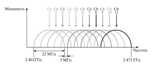
Рис. 3.10 Каналы, используемые в технологии DSSS
Беспроводные локальные сети DSSS используют каналы шириной 22 МГц, благодаря чему многие WLAN могут работать в одной и той же зоне покрытия. В Северной Америке и большей части Европы, в том числе и в России, каналы шириной 22 МГц позволяют создать в диапазоне 2,4- 2,483 ГГц три неперекрывающихся канала передачи. Эти каналы показаны на Рис. 3.10.
Существует три наиболее распространенных орудия борьбы с ошибками в процессе передачи данных:
1.коды обнаружения ошибок;
2.коды с коррекцией ошибок, называемые также схемами прямой коррекции ошибок (Forward Error Correction — FEC);
3.протоколы с автоматическим запросом повторной передачи (Automatic Repeat Request
— ARQ).
Код обнаружения ошибок позволяет довольно легко установить наличие ошибки. Как правило, подобные коды используются совместно с определенными протоколами канального или транспортного уровней, имеющими схему ARQ. В схеме ARQ приемник попросту отклоняет блок данных, в котором была обнаружена ошибка, после чего передатчик передает этот блок повторно. Коды с прямой коррекцией ошибок позволяют не только обнаружить ошибки, но и исправить их, не прибегая к повторной передаче. Схемы FEC часто используются в беспроводной передаче, где повторная передача крайне неэффективна, а уровень ошибок довольно высок.
Методы обнаружения ошибок
Методы обнаружения ошибок основаны на передаче в составе блока данных избыточной служебной информации, по которой можно судить с некоторой степенью вероятности о достоверности принятых данных.
Избыточную служебную информацию принято называть контрольной суммой, или контрольной последовательностью кадра (Frame Check Sequence, FCS). Контрольная сумма вычисляется как функция от основной информации, причем не обязательно путем суммирования. Принимающая сторона повторно вычисляет контрольную сумму кадра по известному алгоритму и в случае ее совпадения с контрольной суммой, вычисленной передающей стороной, делает вывод о том, что данные были переданы через сеть корректно. Рассмотрим несколько распространенных алгоритмов вычисления контрольной суммы, отличающихся вычислительной сложностью и способностью обнаруживать ошибки в данных.
Контроль по паритету представляет собой наиболее простой метод контроля данных. В то же время это наименее мощный алгоритм контроля, так как с его помощью можно обнаружить только одиночные ошибки в проверяемых данных. Метод заключается в суммировании по модулю 2 всех битов контролируемой информации. Нетрудно заметить, что для информации, состоящей из нечетного числа единиц, контрольная сумма всегда равна 1, а при четном числе единиц — 0. Например, для данных 100101011 результатом контрольного суммирования будет значение 1. Результат суммирования также представляет собой один дополнительный бит данных, который пересылается вместе с контролируемой информацией. При искажении в процессе пересылки любого бита исходных данных (или контрольного разряда) результат суммирования будет отличаться от принятого контрольного разряда, что говорит об ошибке. Однако двойная ошибка, например 110101010, будет неверно принята за корректные данные. Поэтому контроль по паритету применяется к небольшим порциям данных, как правило, к каждому байту, что дает коэффициент избыточности для этого метода 1/8. Метод редко применяется в компьютерных сетях из-за значительной избыточности и невысоких диагностических способностей.
Вертикальный и горизонтальный контроль по паритету представляет собой модификацию описанного выше метода. Его отличие состоит в том, что исходные данные рассматриваются в виде матрицы, строки которой составляют байты данных. Контрольный разряд подсчитывается отдельно для каждой строки и для каждого столбца матрицы. Этот метод обнаруживает значительную часть двойных ошибок, однако обладает еще большей избыточностью. Он сейчас также почти не применяется при передаче информации по сети.
Циклический избыточный контроль (Cyclic Redundancy Check — CRC) является в настоящее время наиболее популярным методом контроля в вычислительных сетях (и не только в сетях; в частности, этот метод широко применяется при записи данных на гибкие и жесткие диски). Метод основан на рассмотрении исходных данных в виде одного многоразрядного двоичного числа. Например, кадр стандарта Ethernet, состоящий из 1024 байт, будет рассматриваться как одно число, состоящее из 8192 бит. Контрольной информацией считается остаток от деления этого числа на известный делитель R. Обычно в качестве делителя выбирается семнадцатиили тридцатитрехразрядное число, чтобы остаток от деления имел длину 16 разрядов (2 байт) или 32 разряда (4 байт). При получении кадра данных снова вычисляется остаток от деления на тот же делитель R, но при этом к данным кадра добавляется и содержащаяся в нем контрольная сумма. Если остаток от деления на R равен нулю, то делается вывод об отсутствии ошибок в полученном кадре, в противном случае кадр считается искаженным.
Этот метод обладает более высокой вычислительной сложностью, но его диагностические возможности гораздо шире, чем у методов контроля по паритету. Метод CRC обнаруживает все одиночные ошибки, двойные ошибки и ошибки в нечетном числе битов. Метод также обладает невысокой степенью избыточности. Например, для кадра Ethernet размером 1024 байта контрольная информация длиной 4 байта составляет только 0,4 %.
Методы коррекции ошибок
Техника кодирования, которая позволяет приемнику не только понять, что присланные данные содержат ошибки, но и исправить их, называется прямой коррекцией ошибок (Forward Error Correction — FEC). Коды, обеспечивающие прямую коррекцию ошибок, требуют введения большей избыточности в передаваемые данные, чем коды, которые только обнаруживают ошибки.
При применении любого избыточного кода не все комбинации кодов являются разрешенными. Например, контроль по паритету делает разрешенными только половину
кодов. Если мы контролируем три информационных бита, то разрешенными 4-битными кодами с дополнением до нечетного количества единиц будут:
000 1, 001 0, 010 0, 011 1, 100 0, 101 1, 110 1, 111 0, то есть всего 8 кодов из 16 возможных. Для того чтобы оценить количество дополнительных битов, необходимых для исправления ошибок, нужно знать так называемое расстояние Хемминга между разрешенными комбинациями кода. Расстоянием Хемминга называется минимальное число битовых разрядов, в которых отличается любая пара разрешенных кодов. Для схем
контроля по паритету расстояние Хемминга равно 2.
Можно доказать, что если мы сконструировали избыточный код с расстоянием Хемминга, равным n, такой код будет в состоянии распознавать (n-1)-кратные ошибки и исправлять (n-1)/2-кратные ошибки. Так как коды с контролем по паритету имеют расстояние Хемминга, равное 2, они могут только обнаруживать однократные ошибки и не могут исправлять ошибки.
Коды Хемминга эффективно обнаруживают и исправляют изолированные ошибки, то есть отдельные искаженные биты, которые разделены большим количеством корректных битов. Однако при появлении длинной последовательности искаженных битов (пульсации ошибок) коды Хемминга не работают.
Наиболее часто в современных системах связи применяется тип кодирования, реализуемый сверточным кодирующим устройством (Сonvolutional coder), потому что такое кодирование несложно реализовать аппаратно с использованием линий задержки (delay) и сумматоров. В отличие от рассмотренного выше кода, который относится к блочным кодам без памяти, сверточный код относится к кодам с конечной памятью (Finite memory code); это означает, что выходная последовательность кодера является функцией не только текущего входного сигнала, но также нескольких из числа последних предшествующих битов. Длина кодового ограничения (Constraint length of a code) показывает, как много выходных элементов выходит из системы в пересчете на один входной. Коды часто характеризуются их эффективной степенью (или коэффициентом) кодирования (Code rate). Вам может встретиться сверточный код с коэффициентом кодирования 1/2. Этот коэффициент указывает, что на каждый входной бит приходится два выходных. При сравнении кодов обращайте внимание на то, что, хотя коды с более высокой эффективной степенью кодирования позволяют передавать данные с более высокой скоростью, они, соответственно, более чувствительны к шуму.
В беспроводных системах с блочными кодами широко используется метод чередования блоков. Преимущество чередования состоит в том, что приемник распределяет пакет ошибок, исказивший некоторую последовательность битов, по большому числу блоков, благодаря чему становится возможным исправление ошибок. Чередование выполняется с помощью чтения и записи данных в различном порядке. Если во время передачи пакет помех воздействует на некоторую последовательность битов, то все эти биты оказываются разнесенными по различным блокам. Следовательно, от любой контрольной последовательности требуется возможность исправить лишь небольшую часть от общего количества инвертированных битов.
Методы автоматического запроса повторной передачи
В простейшем случае защита от ошибок заключается только в их обнаружении. Система должна предупредить передатчик об обнаружении ошибки и необходимости повторной передачи. Такие процедуры защиты от ошибок известны как методы автоматического запроса повторной передачи (Automatic Repeat Request — ARQ). В беспроводных локальных сетях применяется процедура «запрос ARQ с остановками» (stop-and-wait ARQ).
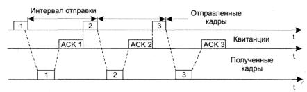
Рис. 3.11 Процедура запрос ARQ с остановками
В этом случае источник, пославший кадр, ожидает получения подтверждения (Acknowledgement — ACK), или, как еще его называют, квитанции, от приемника и только после этого посылает следующий кадр. Если же подтверждение не приходит в течение тайм-аута, то кадр (или подтверждение) считается утерянным и его передача повторяется. На Рис. 3.11 видно, что в этом случае производительность обмена данными ниже потенциально возможной; хотя передатчик и мог бы послать следующий кадр сразу же после отправки предыдущего, он обязан ждать прихода подтверждения.
Соседние файлы в предмете [НЕСОРТИРОВАННОЕ]
- #
- #
- #
- #
- #
- #
- #
- #
- #
- #
- #
Введение
Одной из ключевых задач, решаемых разработчиками любых систем связи (и в первую очередь систем радиосвязи) является задача обнаружения и исправления ошибок, количество которых в сотовых сетях определяется двумя факторами – внешними помехами, а также интерференцией, возникающей от передатчиков соседних базовых станций. Последний фактор является особенно важным для одночастотных систем мобильной связи, включая 4G—LTE и 5G.
Рассмотрим основные технологии и понятия, связанные с решением обозначенной задачи на сетях 4G-LTE и 5G:
Схема с прямой коррекцией ошибок – FEC (Forward Error Correction)
Суть схемы FEC заключается в преобразовании передатчиком передаваемых блоков данных в кодовые слова (путем канального кодирования и внесения избыточной информации) таким образом, чтобы предоставить приемнику возможность обнаруживать и восстанавливать определенное количество битов, искаженных при передаче – см. Рис. 1. Подобные системы характеризуются скоростью кодирования, представляющей собой отношение длины полезного блока данных к длине кодового слова. Недостатком является потеря функциональности при превышении кол-ва ошибок исправляющей способности кода.

Рис. 1 (FEC + Rate matching)
Выравнивание скорости – Rate matching
Выравнивание скорости представляет собой функциональный модуль, дополняющий технологию прямой коррекции ошибок. Данный модуль удаляет (или «выкалывает») часть битов из кодовых слов, формируемых схемой FEC, уменьшая их длину до требуемого размера транспортного блока. Тем самым, с одной стороны снижается объем данных, который передается по каналу связи, с другой – сохраняется достаточная исправляющая способность системы. На приемной стороне в выколотые передатчиком позиции вставляются фиктивные биты, после чего кодовые слова восстановленной длины направляются на канальный декодер.
Схема с автоматическим запросом повторной передачи – ARQ (Automatic Repeat request)
Суть схемы ARQ заключается в вычислении передатчиком циклического избыточного кода (CRC – Cyclic Redundancy Check) передаваемого блока данных, что позволяет приемнику путем сравнения вычисленного и принятого значений CRC обнаруживать пакеты, содержащие искаженные данные и запрашивать их повторную передачу – см. Рис. 2.
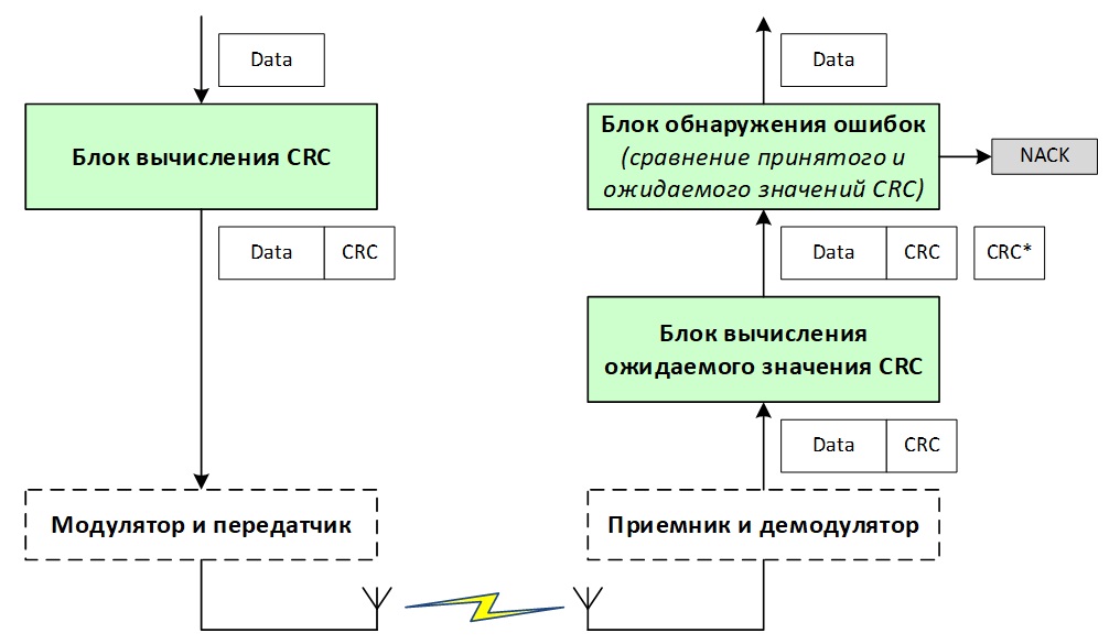
Рис. 2 (ARQ)
Обычно схема ARQ использует метод, называемый выборочной ретрансляцией (Рис. 3), в котором приемник ожидает получение нескольких блоков данных до их подтверждения. Этот метод с одной стороны позволяет передатчику продолжать отправлять пакеты, не дожидаясь их подтверждения, а с другой стороны вносит существенную задержку в случае необходимости повторной передачи. Следовательно, схема ARQ подходит только для потоков данных нереального времени, таких как веб-страницы и электронные письма. Кроме уже упомянутой задержки, недостатком схемы ARQ является дополнительная нагрузка на канал связи, поскольку даже единичная ошибка требует повторной передачи всего пакета данных.

Рис. 3 (метод выборочной ретрансляции ARQ)
Гибридная схема с автоматическим запросом повторной передачи – HARQ (Hybrid ARQ)
Hybrid ARQ комбинирует вышеописанные схемы, применяемые для коррекции ошибок (FEC, ARQ – см. Рис. 4). В соответствии с этим, передающая сторона:
- осуществляет кодирование передаваемых данных FEC кодом (с применением функции выравнивания скорости), что позволяет приемнику восстанавливать искаженные при передаче биты (в пределах исправляющей способности кода);
- вычисляет код CRC и добавляет его к передаваемым данным, давая возможность приемнику детектировать блоки, содержащие неисправленные посредством FEC ошибки, и запрашивать их повторную передачу.

Рис. 4 (HARQ)
Схемы HARQ могут быть синхронными и асинхронными. В синхронном режиме повторная передача блоков данных осуществляется в строго определенные интервалы времени. При этом не требуется передача номера HARQ процесса (см. п.3) и номера Redundancy version (RV – см. п.2), что снижает долю сигнального трафика. Так, каждый субфрейм (sub frame) планировщик базовой станции выделяет ресурс для передачи только одному предопределенному HARQ процессу с предопределенным RV, и в системе, содержащей 8 процессов, каждый процесс осуществляет передачу строго раз в 8мс.
В асинхронном режиме передача данных HARQ процессами может осуществляться в любое время, что дает возможность планировщику базовой станции более гибко распределять ресурсы сети. Плата за эту гибкость – увеличение накладных расходов на передачу сигнальной информации (номер HARQ процесса, а также номер RV включаются в блок управляющей информации – DCI, передаваемый по каналу PDCCH).
На восходящих линиях (Uplink) сетей 4G—LTE и 5G используется синхронный режим HARQ, на нисходящей (Downlink) – асинхронный.
Также алгоритмы HARQ могут функционировать в адаптивном и неадаптивном режимах. В адаптивном режиме при повторной передаче пакетов допускается изменение таких параметров как скорость кодирования, номера и кол-во выделенных ресурсных блоков, схема модуляции. По аналогии с асинхронной передачей адаптивный режим повышает гибкость распределения ресурсов сети, предоставляет механизмы для увеличения надежности приема данных (например, за счет понижения индекса модуляции), но при этом увеличивает долю сигнального трафика на канале PDCCH.
Неадаптивный режим не предполагает изменения параметров при повторной передаче пакетов.