Метод обратного распространения ошибки
Термин
«обратное распространение» относится
к процессу, с помощью которого могут
быть вычислены производные функционала
ошибки по параметрам сети. Этот процесс
может использоваться в сочетании с
различными стратегиями оптимизации.
Существует много вариантов и самого
алгоритма обратного распространения.
Обратимся к одному из них.
Рассмотрим выражение для градиента
критерия качества по весовым коэффициентам
для выходного слоя M:
 (3.9)
(3.9)
где
 –
–
число нейронов в слое; –k-й элемент вектора выхода слояM
для элемента выборки с номеромq.
Правило функционирования слоя M:
 (3.10)
Из уравнения (3.8) следует
 (3.11)
После подстановки (3.11) в (3.9) имеем:

Если обозначить
 (3.12)
то получим
 (3.13)
Перейдем к выводу соотношений для
настройки весов
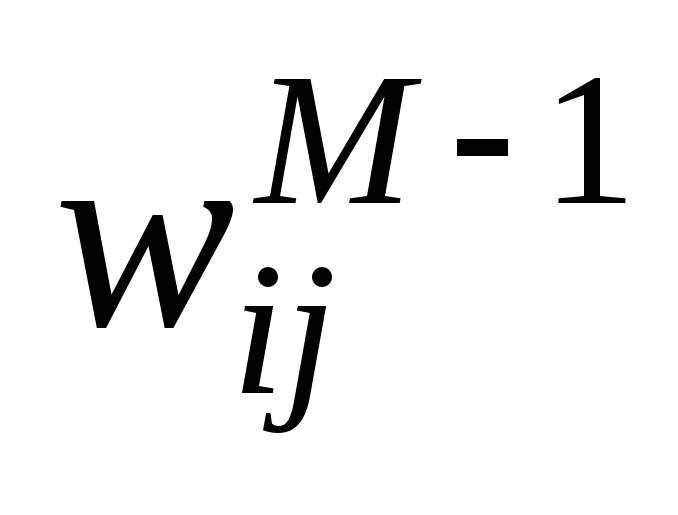 слояM–1
 (3.14)
где

Для слоев M–2,M–3,
…,1 вычисление частных производных
критерияJпо элементам
матриц весовых коэффициентов выполняется
аналогично. В итоге получаем следующую
общую формулу:
 (3.15)
где r– номер слоя

На рис. 3.6 представлена схема вычислений,
соответствующая выражению (3.15).
 Рис. 3.6
На этой схеме символом * обозначена
операция поэлементного умножения
векторов, а символом ** – умножение
вектора наaT;
символ, обозначающий номер элемента
выборки, для краткости опущен.
Характеристика методов обучения
Методы,
используемые при обучении нейронных
сетей, во многом аналогичны методам
определения экстремума функции нескольких
переменных. В свою очередь, последние
делятся на 3 категории – методы нулевого,
первого и второго порядка.
В методах нулевого порядкадля
нахождения экстремума используется
только информация о значениях функции
в заданных точках.
В методах первого порядкаиспользуетсяградиент функционала ошибкипо
настраиваемым параметрам
 (3.16)
где
 – вектор параметров;
 – параметр скорости обучения;
 –
–
градиент функционала, соответствующие
итерации с номеромk.
Вектор в направлении, противоположном
градиенту, указывает направление
кратчайшего спуска по поверхности
функционала ошибки. Если реализуется
движение в этом направлении, то ошибка
будет уменьшаться. Последовательность
таких шагов в конце концов приведет к
значениям настраиваемых параметров,
обеспечивающим минимум функционала.
Определенную трудность здесь вызывает
выбор параметра скорости обучения
 .
.
При большом значении параметра сходимость будет быстрой, но существует
опасность пропустить решение или уйти
в неправильном направлении. Классическим
примером является ситуация, когда
алгоритм очень медленно продвигается
по узкому оврагу с крутыми склонами,
перепрыгивая с одного на другой. Напротив,
при малом шаге, вероятно, будет выбрано
верное направление, однако при этом
потребуется очень много итераций. В
зависимости от принятого алгоритма
параметр скорости обучения может быть
постоянным или переменным. Правильный
выбор этого параметра зависит от
конкретной задачи и обычно осуществляется
опытным путем; в случае переменного
параметра его значение уменьшается по
мере приближения к минимуму функционала.
В алгоритмах сопряженного градиента[12] поиск минимума выполняется вдоль
сопряженных направлений, что
обеспечивает обычно более быструю
сходимость, чем
при наискорейшем
спуске. Все алгоритмы сопряженных
градиентов на первой итерации начинают
движение в направлении антиградиента
 (3.17)
Тогда
направление следующего движения
определяется так, чтобы оно было сопряжено
с предыдущим.
Соответствующее выражение для нового
направления движения является комбинацией
нового направления наискорейшего спуска
и предыдущего направления:
 (3.18)
Здесь
 – направление движения,
 –
–
градиент функционала ошибки, – коэффициент соответствуют итерации
с номеромk. Когда направление спуска
определено,
то новое значение вектора
настраиваемых параметров вычисляется по формуле
 . (3.19)
Методы второго порядка требуют
знания вторых производных функционала
ошибки.
К методам второго порядка
относится метод Ньютона. Основной шаг
метода Ньютона определяется по формуле
 , (3.20)
где
 – вектор значений параметров наk-й
итерации; H– матрица вторых частных
производных целевой функции, или матрица
Гессе; – вектор градиента наk-й итерации.
Во многих случаях метод Ньютона сходится
быстрее, чем методы сопряженного
градиента, но требует больших затрат
из-за вычисления гессиана. Для того
чтобы избежать вычисления матрицы
Гессе, предлагаются различные способы
ее замены приближенными выражениями,
что порождает так называемыеквазиньютоновыалгоритмы(алгоритм метода секущих
плоскостей OSS [1], алгоритм LM Левенберга
– Марквардта [17]).
Соседние файлы в предмете [НЕСОРТИРОВАННОЕ]
- #
- #
- #
- #
- #
- #
- #
- #
- #
- #
- #
Backpropagation-Matlab
Classifying MNIST Handwritten Images using ANN Backpropagation algorithm in Matlab
In this assignment we worked with the MNIST database of 60k handwritten training images and 10k test images. Using a two layer ANN with log-sigmoid transfer functions and backpropagation we trained our network on the training images in order to classify the handwritten digits. Our code includes ten target pattern outputs (0 through 9). We increased our hidden units to 50, and modified our learning rate to 0.00005. As stated on the MNIST databse website, the test images are half normal random samples from the training set, and half distorted digits. Because of this we broke the 10k test images into two categories: 5k for “test images” and 5k for “distorted test images”. The training happens in the main loop which represents one single epoch. During each epoch we complete the forward pass with the training images, the testing of both the normal and distorted test images, and finally the backward pass to update the weights and bias’. During the backpropagation training we stored the error values for the training set and divided test set images in vectors, then took the mean in order to observe the mean squared error and epoch relationship seen below in figure 1.
Fig 1: Backpropagation Training Results with 50 Hidden Units

The results of our backpropagation training show that the mean squared error for the training and normal test images is nearly identical during each epoch. This is expected since the patterns are not distorted. We can also see that the distorted test images have a slightly higher MSE and reach a mean squared error around 1.5 after the tenth epoch. These results were not surprising to us since the distorted images are more prone to incorrect classification.
The aspect of this ANN architecture that we chose to explore was the number of hidden units. Our original number of hidden units was 50 and the results of the network’s performance can be seen above in figure 1. When modifying the number of hidden units to higher numbers, such as 100, 500 and 1k hidden units, the network’s performance with the test set produced a higher MSE. These results can be seen in the figures 2, 3, and 4 below.
Fig 2: Backpropagation Training Results with 100 Hidden Units

Fig 3: Backpropagation Training Results with 500 Hidden Units

Fig 4: Backpropagation Training Results with 1000 Hidden Units

Overall, the relationship between the hidden units, the learning process, and the resultant network’s performance on the test set show that with a higher number of hidden units the MSE will increase. This relationship is also true for the distorted test images which show in the above figures that the MSE increases as the number of hidden units increases.
Backpropagation-Matlab
Classifying MNIST Handwritten Images using ANN Backpropagation algorithm in Matlab
In this assignment we worked with the MNIST database of 60k handwritten training images and 10k test images. Using a two layer ANN with log-sigmoid transfer functions and backpropagation we trained our network on the training images in order to classify the handwritten digits. Our code includes ten target pattern outputs (0 through 9). We increased our hidden units to 50, and modified our learning rate to 0.00005. As stated on the MNIST databse website, the test images are half normal random samples from the training set, and half distorted digits. Because of this we broke the 10k test images into two categories: 5k for “test images” and 5k for “distorted test images”. The training happens in the main loop which represents one single epoch. During each epoch we complete the forward pass with the training images, the testing of both the normal and distorted test images, and finally the backward pass to update the weights and bias’. During the backpropagation training we stored the error values for the training set and divided test set images in vectors, then took the mean in order to observe the mean squared error and epoch relationship seen below in figure 1.
Fig 1: Backpropagation Training Results with 50 Hidden Units
The results of our backpropagation training show that the mean squared error for the training and normal test images is nearly identical during each epoch. This is expected since the patterns are not distorted. We can also see that the distorted test images have a slightly higher MSE and reach a mean squared error around 1.5 after the tenth epoch. These results were not surprising to us since the distorted images are more prone to incorrect classification.
The aspect of this ANN architecture that we chose to explore was the number of hidden units. Our original number of hidden units was 50 and the results of the network’s performance can be seen above in figure 1. When modifying the number of hidden units to higher numbers, such as 100, 500 and 1k hidden units, the network’s performance with the test set produced a higher MSE. These results can be seen in the figures 2, 3, and 4 below.
Fig 2: Backpropagation Training Results with 100 Hidden Units
Fig 3: Backpropagation Training Results with 500 Hidden Units
Fig 4: Backpropagation Training Results with 1000 Hidden Units
Overall, the relationship between the hidden units, the learning process, and the resultant network’s performance on the test set show that with a higher number of hidden units the MSE will increase. This relationship is also true for the distorted test images which show in the above figures that the MSE increases as the number of hidden units increases.
Like the quasi-Newton methods, the Levenberg-Marquardt algorithm was designed to approach second-order training speed
without having to compute the Hessian matrix. When the performance function has the form of a
sum of squares (as is typical in training feedforward networks), then the Hessian matrix can be
approximated as
and the gradient can be computed as
where J is the Jacobian matrix that contains first derivatives of the network errors with respect
to the weights and biases, and e is a vector of network
errors. The Jacobian matrix can be computed through a standard backpropagation technique (see
[HaMe94]) that is much less complex than computing the Hessian
matrix.
The Levenberg-Marquardt algorithm uses this approximation to the Hessian matrix in the
following Newton-like update:
When the scalar µ is zero, this is just Newton’s method, using the approximate Hessian matrix. When µ is
large, this becomes gradient descent with a small step size. Newton’s method is faster and more
accurate near an error minimum, so the aim is to shift toward Newton’s method as quickly as
possible. Thus, µ is decreased after each successful step (reduction in
performance function) and is increased only when a tentative step would increase the
performance function. In this way, the performance function is always reduced at each iteration
of the algorithm.
The original description of the Levenberg-Marquardt algorithm is given in [Marq63]. The application of Levenberg-Marquardt to neural network
training is described in [HaMe94] and starting on page 12-19
of [HDB96]. This algorithm appears to be the fastest method for
training moderate-sized feedforward neural networks (up to several hundred weights). It also
has an efficient implementation in MATLAB® software, because
the solution of the matrix equation is a built-in function, so its attributes become even more
pronounced in a MATLAB environment.
Try the Neural Network Design
demonstration nnd12m [HDB96] for an illustration of the performance of the batch
Levenberg-Marquardt algorithm.
Like the quasi-Newton methods, the Levenberg-Marquardt algorithm was designed to approach second-order training speed
without having to compute the Hessian matrix. When the performance function has the form of a
sum of squares (as is typical in training feedforward networks), then the Hessian matrix can be
approximated as
and the gradient can be computed as
where J is the Jacobian matrix that contains first derivatives of the network errors with respect
to the weights and biases, and e is a vector of network
errors. The Jacobian matrix can be computed through a standard backpropagation technique (see
[HaMe94]) that is much less complex than computing the Hessian
matrix.
The Levenberg-Marquardt algorithm uses this approximation to the Hessian matrix in the
following Newton-like update:
When the scalar µ is zero, this is just Newton’s method, using the approximate Hessian matrix. When µ is
large, this becomes gradient descent with a small step size. Newton’s method is faster and more
accurate near an error minimum, so the aim is to shift toward Newton’s method as quickly as
possible. Thus, µ is decreased after each successful step (reduction in
performance function) and is increased only when a tentative step would increase the
performance function. In this way, the performance function is always reduced at each iteration
of the algorithm.
The original description of the Levenberg-Marquardt algorithm is given in [Marq63]. The application of Levenberg-Marquardt to neural network
training is described in [HaMe94] and starting on page 12-19
of [HDB96]. This algorithm appears to be the fastest method for
training moderate-sized feedforward neural networks (up to several hundred weights). It also
has an efficient implementation in MATLAB® software, because
the solution of the matrix equation is a built-in function, so its attributes become even more
pronounced in a MATLAB environment.
Try the Neural Network Design
demonstration nnd12m [HDB96] for an illustration of the performance of the batch
Levenberg-Marquardt algorithm.