
Лабораторная работа №4
Сравнение групп Критерий Стьюдента Краткие сведения из теории
Результатом исследования обычно является
утверждение, имеющее важное значение,
например, какой метод лучше для лечения
болезни, каковы самые распространенные
побочные эффекты определенного вида
хирургического вмешательства, каков
коэффициент выживаемости после
определенного лечения и действительно
ли новое экспериментальное лекарство
улучшает состояние организма.
Однако, прежде чем получить результат
(утверждение или вывод), необходимо
правильно cпланировать
ход исследования, одним из важных этаповявляется формулировка исходного
утверждения, правильность которого
и проверяется в ходе исследования.
Такое утверждение называетсягипотезой.
Гипотеза —
утверждение, предполагающее доказательство
Проверка гипотезы— это статистическая
процедура, предназначенная для проверки
утверждения. Обычно утверждение касается
исследуемогопараметрасовокупности (т.е. некой величины, которая
характеризует какую-то интересующую
нас сторону объекта).
К примеру, среднее
время госпитализации у первой исследуемой
группы составило 4,5 суток, у второй –
6,3 суток (переменная– время
госпитализации,параметр–
среднее значение дней госпитализации).
В этом примере под гипотезой может
выступать утверждение: различие между
средними значениями статистически
значимо
После того как исследователь определил
переменную и параметр, влияние, на
которые того или иного фактора проверяется
в исследовании, он формулирует нулевую
гипотезу.
Например, при лечении
пациентов согласно официальным схемам
лечения (первая группа) и лечение той
же болезни, но не согласующееся полностью
с официальными схемами (вторая группа)
среднее время госпитализации составило:
у первой исследуемой группы 4,5 суток, у
второй – 6,3 суток. В этом случае влияющий
фактор – лечение согласно официальным
схемам лечения. Анулевая гипотеза:
различие между группами является
случайным и статистически незначимо
Нулевая гипотеза— это предположение,что исследуемые факторы не оказывают
никакого влияния на измеряемый признак
и полученные различия (исследуемых
параметров, средних значений
количества суток госпитализации у двух
групп выше) случайны.
Например, сравнивая
различающиеся средние значения
артериального давления при применении
двух разных анестетиков, мы выдвигаем
нулевую гипотезу о том, что полученные
различия случайны и значимой разницы
между двумя анестетиками нет
Статистическая
значимость результатов. Уровень
значимости
Получив результат, исследователь делает
вывод о том, значим ли полученный
результат с точки зрения статистического
анализа. Другими словами он делает вывод
о статистической значимостиполученного результата.
Для того, чтобы сделать вывод о наличии
или отсутствии статистической значимости
используется так называемый критерий
значимости.
Полученное числовое
значение критерия значимости указывает
на то, принимается или отвергается
нулевая гипотеза. Однако, выводво многомзависити от того с
какой вероятностью мы можем получить
наблюдаемые результаты при верности
нулевой гипотезы
Статистическое исследование всегда
допускает возможное наличие ошибки, и
необходимо учитывать максимальную
вероятность ее возникновения. Если эта
вероятность мала, то нулевая
гипотезаотвергаетсяи делаетсязаключение о значимостиполученного
результата (например, различие средних
значений двух групп статистически
значимо и не обусловлено случайностью)
Максимальную приемлемую
вероятность отвергнуть верную нулевую
гипотезу называют уровнем значимостии обозначаютα (альфа).
Обычно принимают α = 0,05 (5%). Однако
эта величина может быть и другой: 0,01
(1%), 0,1(10%) и т.д. в зависимости от строгости
исследования.
Если в ходе исследования мы получили
результат, который отвергает нулевую
гипотезу, при уровне значимости 5%, то
можно сказать следующее: если бы
нулевая гипотеза была справедлива, то
вероятность получить наблюдаемые
результаты была бы меньше 5%. В принятой
системе обозначений это записывается
как Р < 0,05.Р есть вероятность ошибочно
отвергнуть нулевую гипотезу. Это еще
не означает что влияние изучаемых
факторов доказано (это вопрос тесно
связан с планированием эксперимента),
но, в тоже время, маловероятно, что
результат обусловлен случайностью.
Стандартное заключение
может выглядеть следующим образом:
нулевая гипотеза об отсутствиивлияния исследуемого препарата, например,
на давление, вряд ли справедлива, иразличия между группами статистически
значимы при 5% уровне значимости.
Разумеется, этот вывод по сути своей
носит вероятностный характер. Не
исключено, что ошибочно признается
неэффективный препарат эффективным,
то есть находятся различия там, где их
нет. Однако можно утверждать, что
вероятность подобной ошибкине
превышает 5%
Критерий
Стьюдента
Критерий Стьюдента используется для
сравнения только двух групп. Это частный
случай дисперсионного анализа. Критерий
Стьюдента чрезвычайно популярен, он
используется более чем в половине
медицинских публикаций.
Следует помнить,
что критерий Стьюдента предназначен
для сравнения только двухгрупп, а
не нескольких групп попарно
Ошибочное использование критерия
Стьюдента увеличивает вероятность
«выявить» не существующие различия.
Например, вместо того
чтобы признать несколькометодов
лечения равно эффективными (или
неэффективными), один из них объявляют
«лучшим».
Общая формула для вычисления критерия
Стьюдента:

Для двух случайных выборок извлеченных
из одной нормально распределенной
совокупности это отношение, как правило,
будет близко к нулю.Чем меньше (по
абсолютной величине, по модулю) t, тем
больше вероятность справедливости
нулевой гипотезы. Чем больше t, тем больше
оснований отвергнуть нулевую гипотезу
и считать, что различия статистически
значимы.Величина критерия Стьюдента,
начиная с которойотвергаетсянулевая гипотеза, называетсякритическим
значениемкритерия Стьюдента (tкр).
Если значение tкритерия Стьюдента по модулюбольшечемкритическое значение критерия
Стьюдента(найденное по таблице
критических значений или рассчитанное
при помощи программного обеспечения)
длязаданного уровня значимости,
то нулевая гипотезаотвергается,
и различия считаютсястатистически
значимыми
Это означает, что если бы группы
представляли собой две случайные выборки
из одной и той же совокупности, то
вероятность получить наблюдаемые
различия (или более сильные) равна 0,05
(или другому значению выбранного уровня
значимости).Следовательно, ошибочный
вывод о существовании различий мы будем
делать в 5% случаев.Застраховаться
от подобных ошибок можно приняв уровень
значимости не 0,05, а к примеру 0,01. Однако
даже в этом случае ошибочные выводы о
существовании различий все же не
исключены — их вероятность снижается
до 1% и в тоже время вероятность не найти
различии там где они есть теперь
повысилась.
Ошибки
в использовании критерия Стьюдента
Критерий Стьюдента предназначен для
сравнения двух групп. Однако на практике
он широко используется для оценки
различий большего числа групп посредством
попарного их сравнения. При этом вступает
в силу эффект множественных сравнений.
Пример
Исследуется
влияние препаратов А и Б на уровень
глюкозы плазмы. Исследование проводят
на трех группах — получавших препарат
А, получавших препарат Б и получавших
плацебо В. С помощью критерия Стьюдента
проводят 3 парных сравнения: группу А
сравнивают с группой В, группу Б — с
группой В и наконец А с Б. Получив
достаточно высокое значение t в каком
либо из трех сравнении сообщают что «P
< 0,05». Это означает, что вероятность
ошибочного заключения о существовании
различии не превышает 5%. Но это неверно:
вероятность ошибки значительно превышает
5%. Разберемся подробнее. В исследовании
был принят 5% уровень значимости. Значит,
вероятность ошибиться при сравнении
групп А и В — 5%. Казалось бы все правильно.
Но точно также мы ошибемся в 5% случаев
при сравнении групп Б и В. И наконец при
сравнении групп А и Б ошибка возможна
также в 5% случаев. Следовательно,
вероятность ошибиться хотя бы в одном
из трех сравнении составит не 5%, а
значительно больше. Итак, в нашем
исследовании вероятность ошибиться
хотя бы в одном из сравнений составляет
примерно 15%. При сравнении четырех групп
число пар и соответственно возможных
попарных сравнений равно 6. Поэтому при
уровне значимости в каждом из сравнений
0,05 вероятность ошибочно обнаружить
различие хотя бы в одном равна уже не
0,05, а примерно 6 × 0,05 = 0,30. И когда
исследователь, выявив таким способом
«эффективный» препарат будет говорить
про 5% вероятность ошибки, на самом деле
эта вероятность равна 30%.
Правила использования
критерия Стьюдента:
• Критерий Стьюдента
может быть использован только в случае
выборок с нормально распределеннымизначениями признака;
• Критерий Стьюдента
может быть использован для проверки
гипотезы о различии средних только
для двух групп;
• Если схема
эксперимента предполагает большее
число групп, необходимо воспользоваться
дисперсионным анализом;
• Если критерии
Стьюдента был использован для проверки
различий между несколькими группами,
то истинный уровень значимости можно
получить, умножив уровень значимости,
приводимый авторами на число возможных
сравнений
-
Общая последовательность
действий при использовании критерия
Стьюдента:
-
Формирование таблиц результатов
измерения (записываются и организуются
в таблицу исследуемые показатели первой
группы и показатели второй группы) -
Выполняется анализ полученных данных
(описательная статистика) -
Проверка соответствия распределения
данных нормальному закону распределения -
Выбирается значение уровня значимости
(в зависимости от строгости исследования:
0,1 или 0,05 или 0,01) -
Формулируется нулевая гипотеза (различие
между группами незначимо или является
следствием случайности) -
Рассчитывается значение критерия
Стьюдента t(значение
критерия, начиная с которого мы отвергаем
нулевую гипотезу) и вероятность
ошибочного результатаP(вероятность ошибочно отвергнуть верную
нулевую гипотезу, то есть найти различия
там, где их нет) -
На основании значения уровня значимости
и количества элементов выборки
определяется величина критического
значения критерия tкр
(значение критерия, начиная с которого
мы отвергаем нулевую гипотезу). -
Сравниваются между собой tиtкр, а такжеPи α, еслиt>tкр
иP< α, то нулевая
гипотеза отвергается и различия между
группами статистически значимы, в
противном случае различия – случайны
или незначимы. Следует учитывать, что
даже при обнаруженной статистической
значимости различий исследователь
может ошибаться, но допустимая вероятность
равна уровню значимости.
-
Задача
Т-критерий Стьюдента (t-тест) простым языком
Сегодня мы говорим о t-критерии. Т-критерий наиболее популярный статистический тест в биомедицинских исследованиях. Также его называют парный Т-критерий Стьюдента, t-test, two-sample unpaired t-test. Однако, при использовании этого статистического инструмента допускается достаточно много ошибок. Сегодня в этой статье мы постараемся разобраться, как избежать ошибок применения t-критерия Стьюдента, как интерпретировать его результаты и как рассчитывать t-критерий самостоятельно. Об этом обо всем читайте далее.
При описании любого статистического критерия, будь то t-критерий Стьюдента, либо какой-либо еще, нужно вспомнить о том, как же вообще используются статистические критерии. Для того, чтобы понять, как используется любой критерий, нужно перейти к нескольким достаточно логичным для понимания этапам:
Этапы статистического вывода (statistic inference)
- Первый из них – это вопрос, который мы хотим изучить с помощью статистических методов. То есть первый этап: что изучаем? И какие у нас есть предположения относительно результата? Этот этап называется этап статистических гипотез.
- Второй этап – нужно определиться с тем, какие у нас есть в реальности данные для того, чтобы ответить на первый вопрос. Этот этап – тип данных.
- Третий этап состоит в том, чтобы выбрать корректный для применения в данной ситуации статистический критерий.
- Четвертый этап это логичный этап применения интерпретации любой формулы, какие результаты мы получили.
- Пятый этап это создание, синтез выводов относительно первого, второго, третьего, четвертого, пятого этапа, то есть что же получили и что же это в реальности значит.
Предлагаю долго не ходить вокруг да около и посмотреть применение t-критерия Стьюдента на реальном примере.
Видео-версия статьи
Пример использования т-критерия Стьюдента
А пример будет достаточно простой: мне интересно, стали ли люди выше за последние 100 лет. Для этого нужно подобрать некоторые данные. Я обнаружил интересную информацию в достаточно известной статье The Guardian (Tall story’s men and women have grown taller over last century, Study Shows (The Guardian, July 2016), которая сравнивает средний возраст человека в разных странах в 1914 году и в аналогичных странах в 2014 году.
Там приведены данные практически по всем государствам. Однако, я взял лишь 5 стран для простоты вычислений: это Россия, Германия, Китай, США и ЮАР, соответственно 1914 год и 2014 год.
Общее количество наблюдений – 5 в 1914 году в группе 1914 года и общее значение также 5 в 2014 году. Будем думать опять же для простоты, что эти данные сопоставимы, и с ними можно работать.
Дальше нужно выбрать критерии – критерии, по которым мы будем давать ответ. Равны ли средние по росту в 1914 году x̅1914 и в 2014 году x̅2014. Я считаю, что нет. Поэтому моя гипотеза это то, что они не равны (x̅1914≠x̅2014). Соответственно альтернативная гипотеза моему предположению, так называемая нулевая гипотеза (нулевая гипотеза консервативна, обратная вашей, часто говорит об отсутствии статистически значимых связей/зависимостей) будет говорить о том, что они между собой на самом деле равны (x̅1914=x̅2014), то есть о том, что все эти находки случайны, и я, по сути, не прав.
Теперь нужно дать какой-то аргументированный ответ. Даем его с помощью статистического критерия. Соответственно теперь наступает самое важное: как выбрать статистический критерий? Я думаю, это будет темой отдельной статьи. Для корректности использования t-критерия Стьюдента лишь скажу, что нужно, чтобы:
Условия применения статистического критерия т-теста (критерия Стьюдента)
— данные распределялись по закону нормального распределения;
— данные были количественными;
— и это две независимые между собой выборки (независимые это значит, что в этих группах разные люди, а никак, например, до и после применения препарата у одной группы, люди должны быть разными, тогда группы являются несвязанными, либо независимыми), этот аспект стоит учитывать для выбора вида т-критерия Стьюдента, так как для парных выборок существует свой парный т-критерий (paired t-test).
В итоге Мы определились с тем, что это будет t-критерий Стьюдента.
Формула t-критерия Стьюдента достаточно простая. Она гласит о том, что в числителе у нас разница средних, в знаменателе у нас корень квадратный суммы ошибок репрезентативности по этим группам:
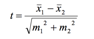
Ошибки репрезентативности были подробно объяснены мною в статье по доверительным интервалам. Поэтому я рекомендую вам ознакомиться с ней, чтобы лучше разобраться, что такое ошибки репрезентативности, что такое выборка, как она соотносится с генеральной совокупностью.
Для того, чтобы не тратить время, я в принципе все уже рассчитал по каждой из групп: средняя (x̅) ,стандартное отклонение (SD) и ошибка репрезентативности (mr).
Давайте остановимся на том, что же значат эти значения:
— средняя (x̅) это среднеарифметическое по 5 наблюдениям в каждой группе;
— если совсем упрощать значение стандартного отклонения (SD), то можно сказать, что оно представляет собой обобщенную среднюю отклонения каждого значения от среднего (стандартное отклонение показывает, насколько широко значения рассеяны (разбросаны) относительно средней). И дальше мы находим нечто среднее отклонений каждого варианта в группе от среднего;
— и ошибка репрезентативности она тоже находится достаточно просто: это как раз наше отклонение от средней некоторое стандартизованное, поэтому стандартное отклонение на размер выборки (mr=).
Итак, продолжаем. В ходе подстановки каждого значения в нашу формулу, мы находим, что t-критерий Стьюдента равен 3,78. Однако, я думаю, пока тем, кто не знаком со статистическими критериями, это мало о чем говорит.
Итак, теперь настает четвертый этап вопрос интерпретации. Ранее мы получили значение t-критерия в 3,78. Однако, что же это значит? Стоит отметить, что результаты статистических критериев и вообще их интерпретация не говорит о точном «да», либо «нет» в выводе, то есть рост отличается, либо рост не отличается. Всегда это вопрос определенной доли вероятности – доли вероятности ошибиться при констатации положительного результата (речь об ошибке первого рода (I type error, Alpha)). То есть, например, если мы скажем, что средний рост в начале ХХ и в начале XXI века отличаются с долей ошибкой меньше 5 %. Как раз эта величина в 5 % и фиксируется как достаточная для большинства биомедицинских исследований, помните, р больше, либо меньше 0,05.
Итак, как нам перейти от нашей t к р вероятности? Это сделать достаточно просто, стоит лишь воспользоваться табличными значениями t для определенных степеней свободы. Теперь вопрос: как найти эти степени свободы? Но это сделать достаточно просто. Для того, чтобы обнаружить степени свободы для наших групп, нужно лишь сложить количество наблюдений 5 и 5 в нашем случае и вычесть 2. В нашем случае степень свободы равна 8.
Итак, t=3,78, степень свободы равна 8. Переходим в табличное значение и получаем р вероятность – вероятность равна 0,005. То есть вероятность того, что мы ошибаемся при констатации факта различия роста ранее и сейчас, крайне мала – это 0,005 %, не 5 %, а 0,005 %. То есть мы можем говорить с высокой долей достоверности того, что наш рост сейчас в XXI веке и 100 лет назад отличаются.
Вот то, что касается расчета t-критерия Стьюдента и его интерпретации.
На этом наш разговор о t-критерии Стьюдента закончен. Спасибо, что ознакомились с этой статьей. Я очень надеюсь на вашу обратную связь. Пожалуйста, подписывайтесь на наш сайте, ставьте лайки, предлагайте свои темы для следующих выпусков. Спасибо большое за поддержку. С вами был Кирилл Мильчаков. Пока, до новых встреч!

Если Вам понравилась статья и оказалась полезной, Вы можете поделиться ею с коллегами и друзьями в социальных сетях:
A t-test is any statistical hypothesis test in which the test statistic follows a Student’s t-distribution under the null hypothesis. It is most commonly applied when the test statistic would follow a normal distribution if the value of a scaling term in the test statistic were known (typically, the scaling term is unknown and therefore a nuisance parameter). When the scaling term is estimated based on the data, the test statistic—under certain conditions—follows a Student’s t distribution. The t-test’s most common application is to test whether the means of two populations are different.
History[edit]

The term «t-statistic» is abbreviated from «hypothesis test statistic».[1] In statistics, the t-distribution was first derived as a posterior distribution in 1876 by Helmert[2][3][4] and Lüroth.[5][6][7] The t-distribution also appeared in a more general form as Pearson Type IV distribution in Karl Pearson’s 1895 paper.[8] However, the T-Distribution, also known as Student’s t-distribution, gets its name from William Sealy Gosset who first published it in English in 1908 in the scientific journal Biometrika using the pseudonym «Student»[9][10] because his employer preferred staff to use pen names when publishing scientific papers.[11] Gosset worked at the Guinness Brewery in Dublin, Ireland, and was interested in the problems of small samples – for example, the chemical properties of barley with small sample sizes. Hence a second version of the etymology of the term Student is that Guinness did not want their competitors to know that they were using the t-test to determine the quality of raw material (see Student’s t-distribution for a detailed history of this pseudonym, which is not to be confused with the literal term student). Although it was William Gosset after whom the term «Student» is penned, it was actually through the work of Ronald Fisher that the distribution became well known as «Student’s distribution»[12] and «Student’s t-test».
Gosset had been hired owing to Claude Guinness’s policy of recruiting the best graduates from Oxford and Cambridge to apply biochemistry and statistics to Guinness’s industrial processes.[13] Gosset devised the t-test as an economical way to monitor the quality of stout. The t-test work was submitted to and accepted in the journal Biometrika and published in 1908.[14]
Guinness had a policy of allowing technical staff leave for study (so-called «study leave»), which Gosset used during the first two terms of the 1906–1907 academic year in Professor Karl Pearson’s Biometric Laboratory at University College London.[15] Gosset’s identity was then known to fellow statisticians and to editor-in-chief Karl Pearson.[16]
Uses[edit]
The most frequently used t-tests are one-sample and two-sample tests:
- A one-sample location test of whether the mean of a population has a value specified in a null hypothesis.
- A two-sample location test of the null hypothesis such that the means of two populations are equal. All such tests are usually called Student’s t-tests, though strictly speaking that name should only be used if the variances of the two populations are also assumed to be equal; the form of the test used when this assumption is dropped is sometimes called Welch’s t-test. These tests are often referred to as unpaired or independent samples t-tests, as they are typically applied when the statistical units underlying the two samples being compared are non-overlapping.[17]
Assumptions[edit]
[dubious – discuss]
Most test statistics have the form t = Z/s, where Z and s are functions of the data.
Z may be sensitive to the alternative hypothesis (i.e., its magnitude tends to be larger when the alternative hypothesis is true), whereas s is a scaling parameter that allows the distribution of t to be determined.
As an example, in the one-sample t-test
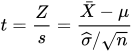
where X is the sample mean from a sample X1, X2, …, Xn, of size n, s is the standard error of the mean, 
The assumptions underlying a t-test in the simplest form above are that:
- X follows a normal distribution with mean μ and variance σ2/n
- s2(n − 1)/σ2 follows a χ2 distribution with n − 1 degrees of freedom. This assumption is met when the observations used for estimating s2 come from a normal distribution (and i.i.d for each group).
- Z and s are independent.
In the t-test comparing the means of two independent samples, the following assumptions should be met:
- The means of the two populations being compared should follow normal distributions. Under weak assumptions, this follows in large samples from the central limit theorem, even when the distribution of observations in each group is non-normal.[18]
- If using Student’s original definition of the t-test, the two populations being compared should have the same variance (testable using F-test, Levene’s test, Bartlett’s test, or the Brown–Forsythe test; or assessable graphically using a Q–Q plot). If the sample sizes in the two groups being compared are equal, Student’s original t-test is highly robust to the presence of unequal variances.[19] Welch’s t-test is insensitive to equality of the variances regardless of whether the sample sizes are similar.
- The data used to carry out the test should either be sampled independently from the two populations being compared or be fully paired. This is in general not testable from the data, but if the data are known to be dependent (e.g. paired by test design), a dependent test has to be applied. For partially paired data, the classical independent t-tests may give invalid results as the test statistic might not follow a t distribution, while the dependent t-test is sub-optimal as it discards the unpaired data.[20]
Most two-sample t-tests are robust to all but large deviations from the assumptions.[21]
For exactness, the t-test and Z-test require normality of the sample means, and the t-test additionally requires that the sample variance follows a scaled χ2 distribution, and that the sample mean and sample variance be statistically independent. Normality of the individual data values is not required if these conditions are met. By the central limit theorem, sample means of moderately large samples are often well-approximated by a normal distribution even if the data are not normally distributed. For non-normal data, the distribution of the sample variance may deviate substantially from a χ2 distribution.
However, if the sample size is large, Slutsky’s theorem implies that the distribution of the sample variance has little effect on the distribution of the test statistic. That is as sample size 
Unpaired and paired two-sample t-tests[edit]
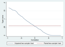
Type I error of unpaired and paired two-sample t-tests as a function of the correlation. The simulated random numbers originate from a bivariate normal distribution with a variance of 1. The significance level is 5% and the number of cases is 60.

Power of unpaired and paired two-sample t-tests as a function of the correlation. The simulated random numbers originate from a bivariate normal distribution with a variance of 1 and a deviation of the expected value of 0.4. The significance level is 5% and the number of cases is 60.
Two-sample t-tests for a difference in means involve independent samples (unpaired samples) or paired samples. Paired t-tests are a form of blocking, and have greater power (probability of avoiding a type II error, also known as a false negative) than unpaired tests when the paired units are similar with respect to «noise factors» that are independent of membership in the two groups being compared.[22] In a different context, paired t-tests can be used to reduce the effects of confounding factors in an observational study.
Independent (unpaired) samples[edit]
The independent samples t-test is used when two separate sets of independent and identically distributed samples are obtained, and one variable from each of the two populations is compared. For example, suppose we are evaluating the effect of a medical treatment, and we enroll 100 subjects into our study, then randomly assign 50 subjects to the treatment group and 50 subjects to the control group. In this case, we have two independent samples and would use the unpaired form of the t-test.
Paired samples[edit]
Paired samples t-tests typically consist of a sample of matched pairs of similar units, or one group of units that has been tested twice (a «repeated measures» t-test).
A typical example of the repeated measures t-test would be where subjects are tested prior to a treatment, say for high blood pressure, and the same subjects are tested again after treatment with a blood-pressure-lowering medication. By comparing the same patient’s numbers before and after treatment, we are effectively using each patient as their own control. That way the correct rejection of the null hypothesis (here: of no difference made by the treatment) can become much more likely, with statistical power increasing simply because the random interpatient variation has now been eliminated. However, an increase of statistical power comes at a price: more tests are required, each subject having to be tested twice. Because half of the sample now depends on the other half, the paired version of Student’s t-test has only n/2 − 1 degrees of freedom (with n being the total number of observations). Pairs become individual test units, and the sample has to be doubled to achieve the same number of degrees of freedom. Normally, there are n − 1 degrees of freedom (with n being the total number of observations).[23]
A paired samples t-test based on a «matched-pairs sample» results from an unpaired sample that is subsequently used to form a paired sample, by using additional variables that were measured along with the variable of interest.[24] The matching is carried out by identifying pairs of values consisting of one observation from each of the two samples, where the pair is similar in terms of other measured variables. This approach is sometimes used in observational studies to reduce or eliminate the effects of confounding factors.
Paired samples t-tests are often referred to as «dependent samples t-tests».
Calculations[edit]
Explicit expressions that can be used to carry out various t-tests are given below. In each case, the formula for a test statistic that either exactly follows or closely approximates a t-distribution under the null hypothesis is given. Also, the appropriate degrees of freedom are given in each case. Each of these statistics can be used to carry out either a one-tailed or two-tailed test.
Once the t value and degrees of freedom are determined, a p-value can be found using a table of values from Student’s t-distribution. If the calculated p-value is below the threshold chosen for statistical significance (usually the 0.10, the 0.05, or 0.01 level), then the null hypothesis is rejected in favor of the alternative hypothesis.
One-sample t-test[edit]
In testing the null hypothesis that the population mean is equal to a specified value μ0, one uses the statistic

where 
Although the parent population does not need to be normally distributed, the distribution of the population of sample means
By the central limit theorem, if the observations are independent and the second moment exists, then 
Slope of a regression line[edit]
Suppose one is fitting the model

where x is known, α and β are unknown, ε is a normally distributed random variable with mean 0 and unknown variance σ2, and Y is the outcome of interest. We want to test the null hypothesis that the slope β is equal to some specified value β0 (often taken to be 0, in which case the null hypothesis is that x and y are uncorrelated).
Let

Then
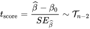
has a t-distribution with n − 2 degrees of freedom if the null hypothesis is true. The standard error of the slope coefficient:
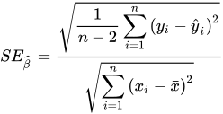
can be written in terms of the residuals. Let

Then tscore is given by:
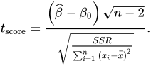
Another way to determine the tscore is:
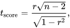
where r is the Pearson correlation coefficient.
The tscore, intercept can be determined from the tscore, slope:
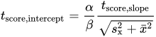
where sx2 is the sample variance.
Independent two-sample t-test[edit]
Equal sample sizes and variance[edit]
Given two groups (1, 2), this test is only applicable when:
- the two sample sizes are equal;
- it can be assumed that the two distributions have the same variance;
Violations of these assumptions are discussed below.
The t statistic to test whether the means are different can be calculated as follows:
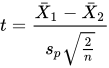
where
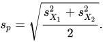
Here sp is the pooled standard deviation for n = n1 = n2 and s 2
X1 and s 2
X2 are the unbiased estimators of the population variance. The denominator of t is the standard error of the difference between two means.
For significance testing, the degrees of freedom for this test is 2n − 2 where n is sample size.
Equal or unequal sample sizes, similar variances (1/2 < sX1/sX2 < 2)[edit]
This test is used only when it can be assumed that the two distributions have the same variance. (When this assumption is violated, see below.)
The previous formulae are a special case of the formulae below, one recovers them when both samples are equal in size: n = n1 = n2.
The t statistic to test whether the means are different can be calculated as follows:
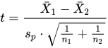
where
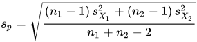
is the pooled standard deviation of the two samples: it is defined in this way so that its square is an unbiased estimator of the common variance whether or not the population means are the same. In these formulae, ni − 1 is the number of degrees of freedom for each group, and the total sample size minus two (that is, n1 + n2 − 2) is the total number of degrees of freedom, which is used in significance testing.
Equal or unequal sample sizes, unequal variances (sX1 > 2sX2 or sX2 > 2sX1)[edit]
This test, also known as Welch’s t-test, is used only when the two population variances are not assumed to be equal (the two sample sizes may or may not be equal) and hence must be estimated separately. The t statistic to test whether the population means are different is calculated as:
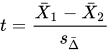
where
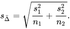
Here si2 is the unbiased estimator of the variance of each of the two samples with ni = number of participants in group i (i = 1 or 2). In this case
is not a pooled variance. For use in significance testing, the distribution of the test statistic is approximated as an ordinary Student’s t-distribution with the degrees of freedom calculated using

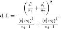
This is known as the Welch–Satterthwaite equation. The true distribution of the test statistic actually depends (slightly) on the two unknown population variances (see Behrens–Fisher problem).
Exact method for unequal variances and sample sizes[edit]
The test[25] deals with the famous Behrens–Fisher problem, i.e., comparing the difference between the means of two normally distributed populations when the variances of the two populations are not assumed to be equal, based on two independent samples.
The test is developed as an exact test that allows for unequal sample sizes and unequal variances of two populations. The exact property still holds even with small extremely small and unbalanced sample sizes (e.g. 
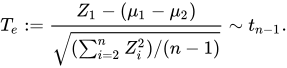
The Te statistic to test whether the means are different can be calculated as follows:
Let ![{displaystyle X=[X_{1},X_{2},ldots ,X_{m}]^{T}}](https://wikimedia.org/api/rest_v1/media/math/render/svg/a0f37f25b326e4b6229a7f0be5283ace07d1a97f)
![{displaystyle Y=[Y_{1},Y_{2},ldots ,Y_{n}]^{T}}](https://wikimedia.org/api/rest_v1/media/math/render/svg/a81b49d1f74f1a3c22759407966c63524eac1d2e)


Let 


Then 

From the above distribution we see that


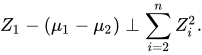
Dependent t-test for paired samples[edit]
This test is used when the samples are dependent; that is, when there is only one sample that has been tested twice (repeated measures) or when there are two samples that have been matched or «paired». This is an example of a paired difference test. The t statistic is calculated as
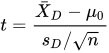
where 

-
Example of repeated measures
Number Name Test 1 Test 2 1 Mike 35% 67% 2 Melanie 50% 46% 3 Melissa 90% 86% 4 Mitchell 78% 91%
-
Example of matched pairs
Pair Name Age Test 1 John 35 250 1 Jane 36 340 2 Jimmy 22 460 2 Jessy 21 200
Worked examples[edit]
Let A1 denote a set obtained by drawing a random sample of six measurements:

and let A2 denote a second set obtained similarly:

These could be, for example, the weights of screws that were chosen out of a bucket.
We will carry out tests of the null hypothesis that the means of the populations from which the two samples were taken are equal.
The difference between the two sample means, each denoted by Xi, which appears in the numerator for all the two-sample testing approaches discussed above, is

The sample standard deviations for the two samples are approximately 0.05 and 0.11, respectively. For such small samples, a test of equality between the two population variances would not be very powerful. Since the sample sizes are equal, the two forms of the two-sample t-test will perform similarly in this example.
Unequal variances[edit]
If the approach for unequal variances (discussed above) is followed, the results are
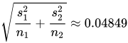
and the degrees of freedom

The test statistic is approximately 1.959, which gives a two-tailed test p-value of 0.09077.
Equal variances[edit]
If the approach for equal variances (discussed above) is followed, the results are
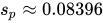
and the degrees of freedom

The test statistic is approximately equal to 1.959, which gives a two-tailed p-value of 0.07857.
[edit]
Alternatives to the t-test for location problems[edit]
The t-test provides an exact test for the equality of the means of two i.i.d. normal populations with unknown, but equal, variances. (Welch’s t-test is a nearly exact test for the case where the data are normal but the variances may differ.) For moderately large samples and a one tailed test, the t-test is relatively robust to moderate violations of the normality assumption.[26] In large enough samples, the t-test asymptotically approaches the z-test, and becomes robust even to large deviations from normality.[18]
If the data are substantially non-normal and the sample size is small, the t-test can give misleading results. See Location test for Gaussian scale mixture distributions for some theory related to one particular family of non-normal distributions.
When the normality assumption does not hold, a non-parametric alternative to the t-test may have better statistical power. However, when data are non-normal with differing variances between groups, a t-test may have better type-1 error control than some non-parametric alternatives.[27] Furthermore, non-parametric methods, such as the Mann-Whitney U test discussed below, typically do not test for a difference of means, so should be used carefully if a difference of means is of primary scientific interest.[18] For example, Mann-Whitney U test will keep the type 1 error at the desired level alpha if both groups have the same distribution. It will also have power in detecting an alternative by which group B has the same distribution as A but after some shift by a constant (in which case there would indeed be a difference in the means of the two groups). However, there could be cases where group A and B will have different distributions but with the same means (such as two distributions, one with positive skewness and the other with a negative one, but shifted so to have the same means). In such cases, MW could have more than alpha level power in rejecting the Null hypothesis but attributing the interpretation of difference in means to such a result would be incorrect.
In the presence of an outlier, the t-test is not robust. For example, for two independent samples when the data distributions are asymmetric (that is, the distributions are skewed) or the distributions have large tails, then the Wilcoxon rank-sum test (also known as the Mann–Whitney U test) can have three to four times higher power than the t-test.[26][28][29] The nonparametric counterpart to the paired samples t-test is the Wilcoxon signed-rank test for paired samples. For a discussion on choosing between the t-test and nonparametric alternatives, see Lumley, et al. (2002).[18]
One-way analysis of variance (ANOVA) generalizes the two-sample t-test when the data belong to more than two groups.
A design which includes both paired observations and independent observations[edit]
When both paired observations and independent observations are present in the two sample design, assuming data are missing completely at random (MCAR), the paired observations or independent observations may be discarded in order to proceed with the standard tests above. Alternatively making use of all of the available data, assuming normality and MCAR, the generalized partially overlapping samples t-test could be used.[30]
Multivariate testing[edit]
A generalization of Student’s t statistic, called Hotelling’s t-squared statistic, allows for the testing of hypotheses on multiple (often correlated) measures within the same sample. For instance, a researcher might submit a number of subjects to a personality test consisting of multiple personality scales (e.g. the Minnesota Multiphasic Personality Inventory). Because measures of this type are usually positively correlated, it is not advisable to conduct separate univariate t-tests to test hypotheses, as these would neglect the covariance among measures and inflate the chance of falsely rejecting at least one hypothesis (Type I error). In this case a single multivariate test is preferable for hypothesis testing. Fisher’s Method for combining multiple tests with alpha reduced for positive correlation among tests is one. Another is Hotelling’s T2 statistic follows a T2 distribution. However, in practice the distribution is rarely used, since tabulated values for T2 are hard to find. Usually, T2 is converted instead to an F statistic.
For a one-sample multivariate test, the hypothesis is that the mean vector (μ) is equal to a given vector (μ0). The test statistic is Hotelling’s t2:

where n is the sample size, x is the vector of column means and S is an m × m sample covariance matrix.
For a two-sample multivariate test, the hypothesis is that the mean vectors (μ1, μ2) of two samples are equal. The test statistic is Hotelling’s two-sample t2:

Software implementations[edit]
Many spreadsheet programs and statistics packages, such as QtiPlot, LibreOffice Calc, Microsoft Excel, SAS, SPSS, Stata, DAP, gretl, R, Python, PSPP, MATLAB and Minitab, include implementations of Student’s t-test.
| Language/Program | Function | Notes |
|---|---|---|
| Microsoft Excel pre 2010 | TTEST(array1, array2, tails, type) |
See [1] |
| Microsoft Excel 2010 and later | T.TEST(array1, array2, tails, type) |
See [2] |
| Apple Numbers | TTEST(sample-1-values, sample-2-values, tails, test-type) |
See [3] |
| LibreOffice Calc | TTEST(Data1; Data2; Mode; Type) |
See [4] |
| Google Sheets | TTEST(range1, range2, tails, type) |
See [5] |
| Python | scipy.stats.ttest_ind(a, b, equal_var=True) |
See [6] |
| MATLAB | ttest(data1, data2) |
See [7] |
| Mathematica | TTest[{data1,data2}] |
See [8] |
| R | t.test(data1, data2, var.equal=TRUE) |
See [9] |
| SAS | PROC TTEST |
See [10] |
| Java | tTest(sample1, sample2) |
See [11] |
| Julia | EqualVarianceTTest(sample1, sample2) |
See [12] |
| Stata | ttest data1 == data2 |
See [13] |
See also[edit]
- Conditional change model
- F-test
- Noncentral t-distribution in power analysis
- Student’s t-statistic
- Z-test
- Mann–Whitney U test
- Šidák correction for t-test
- Welch’s t-test
- Analysis of variance (ANOVA)
References[edit]
Citations[edit]
- ^ The Microbiome in Health and Disease. Academic Press. 2020-05-29. p. 397. ISBN 978-0-12-820001-8.
- ^ Szabó, István (2003), «Systeme aus einer endlichen Anzahl starrer Körper», Einführung in die Technische Mechanik, Springer Berlin Heidelberg, pp. 196–199, doi:10.1007/978-3-642-61925-0_16, ISBN 978-3-540-13293-6
- ^ Schlyvitch, B. (October 1937). «Untersuchungen über den anastomotischen Kanal zwischen der Arteria coeliaca und mesenterica superior und damit in Zusammenhang stehende Fragen». Zeitschrift für Anatomie und Entwicklungsgeschichte. 107 (6): 709–737. doi:10.1007/bf02118337. ISSN 0340-2061. S2CID 27311567.
- ^ Helmert (1876). «Die Genauigkeit der Formel von Peters zur Berechnung des wahrscheinlichen Beobachtungsfehlers directer Beobachtungen gleicher Genauigkeit». Astronomische Nachrichten (in German). 88 (8–9): 113–131. Bibcode:1876AN…..88..113H. doi:10.1002/asna.18760880802.
- ^ Lüroth, J. (1876). «Vergleichung von zwei Werthen des wahrscheinlichen Fehlers». Astronomische Nachrichten (in German). 87 (14): 209–220. Bibcode:1876AN…..87..209L. doi:10.1002/asna.18760871402.
- ^ Pfanzagl J, Sheynin O (1996). «Studies in the history of probability and statistics. XLIV. A forerunner of the t-distribution». Biometrika. 83 (4): 891–898. doi:10.1093/biomet/83.4.891. MR 1766040.
- ^ Sheynin, Oscar (1995). «Helmert’s work in the theory of errors». Archive for History of Exact Sciences. 49 (1): 73–104. doi:10.1007/BF00374700. ISSN 0003-9519. S2CID 121241599.
- ^ Pearson, K. (1895-01-01). «Contributions to the Mathematical Theory of Evolution. II. Skew Variation in Homogeneous Material». Philosophical Transactions of the Royal Society A: Mathematical, Physical and Engineering Sciences. 186: 343–414 (374). doi:10.1098/rsta.1895.0010. ISSN 1364-503X
- ^ «Student» William Sealy Gosset (1908). «The probable error of a mean» (PDF). Biometrika. 6 (1): 1–25. doi:10.1093/biomet/6.1.1. hdl:10338.dmlcz/143545. JSTOR 2331554
- ^ «T Table».
- ^ Wendl MC (2016). «Pseudonymous fame». Science. 351 (6280): 1406. doi:10.1126/science.351.6280.1406. PMID 27013722
- ^ Walpole, Ronald E. (2006). Probability & statistics for engineers & scientists. Myers, H. Raymond. (7th ed.). New Delhi: Pearson. ISBN 81-7758-404-9. OCLC 818811849.
- ^ O’Connor, John J.; Robertson, Edmund F., «William Sealy Gosset», MacTutor History of Mathematics archive, University of St Andrews
- ^ «The Probable Error of a Mean» (PDF). Biometrika. 6 (1): 1–25. 1908. doi:10.1093/biomet/6.1.1. hdl:10338.dmlcz/143545. Retrieved 24 July 2016.
- ^ Raju, T. N. (2005). «William Sealy Gosset and William A. Silverman: Two ‘Students’ of Science». Pediatrics. 116 (3): 732–5. doi:10.1542/peds.2005-1134. PMID 16140715. S2CID 32745754.
- ^ Dodge, Yadolah (2008). The Concise Encyclopedia of Statistics. Springer Science & Business Media. pp. 234–235. ISBN 978-0-387-31742-7.
- ^ Fadem, Barbara (2008). High-Yield Behavioral Science. High-Yield Series. Hagerstown, MD: Lippincott Williams & Wilkins. ISBN 9781451130300.
- ^ a b c d Lumley, Thomas; Diehr, Paula; Emerson, Scott; Chen, Lu (May 2002). «The Importance of the Normality Assumption in Large Public Health Data Sets». Annual Review of Public Health. 23 (1): 151–169. doi:10.1146/annurev.publhealth.23.100901.140546. ISSN 0163-7525. PMID 11910059.
- ^ Markowski, Carol A.; Markowski, Edward P. (1990). «Conditions for the Effectiveness of a Preliminary Test of Variance». The American Statistician. 44 (4): 322–326. doi:10.2307/2684360. JSTOR 2684360.
- ^ Guo, Beibei; Yuan, Ying (2017). «A comparative review of methods for comparing means using partially paired data». Statistical Methods in Medical Research. 26 (3): 1323–1340. doi:10.1177/0962280215577111. PMID 25834090. S2CID 46598415.
- ^ Bland, Martin (1995). An Introduction to Medical Statistics. Oxford University Press. p. 168. ISBN 978-0-19-262428-4.
- ^ Rice, John A. (2006). Mathematical Statistics and Data Analysis (3rd ed.). Duxbury Advanced.[ISBN missing]
- ^ Weisstein, Eric. «Student’s t-Distribution». mathworld.wolfram.com.
- ^ David, H. A.; Gunnink, Jason L. (1997). «The Paired t Test Under Artificial Pairing». The American Statistician. 51 (1): 9–12. doi:10.2307/2684684. JSTOR 2684684.
- ^ Chang Wang, Jinzhu Jia. «A New Non-asymptotic t-test for Behrens-Fisher Problems».https://arxiv.org/abs/2210.16473
- ^ a b Sawilowsky, Shlomo S.; Blair, R. Clifford (1992). «A More Realistic Look at the Robustness and Type II Error Properties of the t Test to Departures From Population Normality». Psychological Bulletin. 111 (2): 352–360. doi:10.1037/0033-2909.111.2.352.
- ^ Zimmerman, Donald W. (January 1998). «Invalidation of Parametric and Nonparametric Statistical Tests by Concurrent Violation of Two Assumptions». The Journal of Experimental Education. 67 (1): 55–68. doi:10.1080/00220979809598344. ISSN 0022-0973.
- ^ Blair, R. Clifford; Higgins, James J. (1980). «A Comparison of the Power of Wilcoxon’s Rank-Sum Statistic to That of Student’s t Statistic Under Various Nonnormal Distributions». Journal of Educational Statistics. 5 (4): 309–335. doi:10.2307/1164905. JSTOR 1164905.
- ^ Fay, Michael P.; Proschan, Michael A. (2010). «Wilcoxon–Mann–Whitney or t-test? On assumptions for hypothesis tests and multiple interpretations of decision rules». Statistics Surveys. 4: 1–39. doi:10.1214/09-SS051. PMC 2857732. PMID 20414472.
- ^ Derrick, B; Toher, D; White, P (2017). «How to compare the means of two samples that include paired observations and independent observations: A companion to Derrick, Russ, Toher and White (2017)» (PDF). The Quantitative Methods for Psychology. 13 (2): 120–126. doi:10.20982/tqmp.13.2.p120.
Sources[edit]
- O’Mahony, Michael (1986). Sensory Evaluation of Food: Statistical Methods and Procedures. CRC Press. p. 487. ISBN 0-82477337-3.
- Press, William H.; Teukolsky, Saul A.; Vetterling, William T.; Flannery, Brian P. (1992). Numerical Recipes in C: The Art of Scientific Computing. Cambridge University Press. p. 616. ISBN 0-521-43108-5.
Further reading[edit]
- Boneau, C. Alan (1960). «The effects of violations of assumptions underlying the t test». Psychological Bulletin. 57 (1): 49–64. doi:10.1037/h0041412. PMID 13802482.
- Edgell, Stephen E.; Noon, Sheila M. (1984). «Effect of violation of normality on the t test of the correlation coefficient». Psychological Bulletin. 95 (3): 576–583. doi:10.1037/0033-2909.95.3.576.
External links[edit]

Wikiversity has learning resources about t-test
- «Student test», Encyclopedia of Mathematics, EMS Press, 2001 [1994]
- Trochim, William M.K. «The T-Test», Research Methods Knowledge Base, conjoint.ly
- Econometrics lecture (topic: hypothesis testing) on YouTube by Mark Thoma
A t-test is any statistical hypothesis test in which the test statistic follows a Student’s t-distribution under the null hypothesis. It is most commonly applied when the test statistic would follow a normal distribution if the value of a scaling term in the test statistic were known (typically, the scaling term is unknown and therefore a nuisance parameter). When the scaling term is estimated based on the data, the test statistic—under certain conditions—follows a Student’s t distribution. The t-test’s most common application is to test whether the means of two populations are different.
History[edit]
The term «t-statistic» is abbreviated from «hypothesis test statistic».[1] In statistics, the t-distribution was first derived as a posterior distribution in 1876 by Helmert[2][3][4] and Lüroth.[5][6][7] The t-distribution also appeared in a more general form as Pearson Type IV distribution in Karl Pearson’s 1895 paper.[8] However, the T-Distribution, also known as Student’s t-distribution, gets its name from William Sealy Gosset who first published it in English in 1908 in the scientific journal Biometrika using the pseudonym «Student»[9][10] because his employer preferred staff to use pen names when publishing scientific papers.[11] Gosset worked at the Guinness Brewery in Dublin, Ireland, and was interested in the problems of small samples – for example, the chemical properties of barley with small sample sizes. Hence a second version of the etymology of the term Student is that Guinness did not want their competitors to know that they were using the t-test to determine the quality of raw material (see Student’s t-distribution for a detailed history of this pseudonym, which is not to be confused with the literal term student). Although it was William Gosset after whom the term «Student» is penned, it was actually through the work of Ronald Fisher that the distribution became well known as «Student’s distribution»[12] and «Student’s t-test».
Gosset had been hired owing to Claude Guinness’s policy of recruiting the best graduates from Oxford and Cambridge to apply biochemistry and statistics to Guinness’s industrial processes.[13] Gosset devised the t-test as an economical way to monitor the quality of stout. The t-test work was submitted to and accepted in the journal Biometrika and published in 1908.[14]
Guinness had a policy of allowing technical staff leave for study (so-called «study leave»), which Gosset used during the first two terms of the 1906–1907 academic year in Professor Karl Pearson’s Biometric Laboratory at University College London.[15] Gosset’s identity was then known to fellow statisticians and to editor-in-chief Karl Pearson.[16]
Uses[edit]
The most frequently used t-tests are one-sample and two-sample tests:
- A one-sample location test of whether the mean of a population has a value specified in a null hypothesis.
- A two-sample location test of the null hypothesis such that the means of two populations are equal. All such tests are usually called Student’s t-tests, though strictly speaking that name should only be used if the variances of the two populations are also assumed to be equal; the form of the test used when this assumption is dropped is sometimes called Welch’s t-test. These tests are often referred to as unpaired or independent samples t-tests, as they are typically applied when the statistical units underlying the two samples being compared are non-overlapping.[17]
Assumptions[edit]
[dubious – discuss]
Most test statistics have the form t = Z/s, where Z and s are functions of the data.
Z may be sensitive to the alternative hypothesis (i.e., its magnitude tends to be larger when the alternative hypothesis is true), whereas s is a scaling parameter that allows the distribution of t to be determined.
As an example, in the one-sample t-test
where X is the sample mean from a sample X1, X2, …, Xn, of size n, s is the standard error of the mean,
The assumptions underlying a t-test in the simplest form above are that:
- X follows a normal distribution with mean μ and variance σ2/n
- s2(n − 1)/σ2 follows a χ2 distribution with n − 1 degrees of freedom. This assumption is met when the observations used for estimating s2 come from a normal distribution (and i.i.d for each group).
- Z and s are independent.
In the t-test comparing the means of two independent samples, the following assumptions should be met:
- The means of the two populations being compared should follow normal distributions. Under weak assumptions, this follows in large samples from the central limit theorem, even when the distribution of observations in each group is non-normal.[18]
- If using Student’s original definition of the t-test, the two populations being compared should have the same variance (testable using F-test, Levene’s test, Bartlett’s test, or the Brown–Forsythe test; or assessable graphically using a Q–Q plot). If the sample sizes in the two groups being compared are equal, Student’s original t-test is highly robust to the presence of unequal variances.[19] Welch’s t-test is insensitive to equality of the variances regardless of whether the sample sizes are similar.
- The data used to carry out the test should either be sampled independently from the two populations being compared or be fully paired. This is in general not testable from the data, but if the data are known to be dependent (e.g. paired by test design), a dependent test has to be applied. For partially paired data, the classical independent t-tests may give invalid results as the test statistic might not follow a t distribution, while the dependent t-test is sub-optimal as it discards the unpaired data.[20]
Most two-sample t-tests are robust to all but large deviations from the assumptions.[21]
For exactness, the t-test and Z-test require normality of the sample means, and the t-test additionally requires that the sample variance follows a scaled χ2 distribution, and that the sample mean and sample variance be statistically independent. Normality of the individual data values is not required if these conditions are met. By the central limit theorem, sample means of moderately large samples are often well-approximated by a normal distribution even if the data are not normally distributed. For non-normal data, the distribution of the sample variance may deviate substantially from a χ2 distribution.
However, if the sample size is large, Slutsky’s theorem implies that the distribution of the sample variance has little effect on the distribution of the test statistic. That is as sample size
Unpaired and paired two-sample t-tests[edit]
Type I error of unpaired and paired two-sample t-tests as a function of the correlation. The simulated random numbers originate from a bivariate normal distribution with a variance of 1. The significance level is 5% and the number of cases is 60.
Power of unpaired and paired two-sample t-tests as a function of the correlation. The simulated random numbers originate from a bivariate normal distribution with a variance of 1 and a deviation of the expected value of 0.4. The significance level is 5% and the number of cases is 60.
Two-sample t-tests for a difference in means involve independent samples (unpaired samples) or paired samples. Paired t-tests are a form of blocking, and have greater power (probability of avoiding a type II error, also known as a false negative) than unpaired tests when the paired units are similar with respect to «noise factors» that are independent of membership in the two groups being compared.[22] In a different context, paired t-tests can be used to reduce the effects of confounding factors in an observational study.
Independent (unpaired) samples[edit]
The independent samples t-test is used when two separate sets of independent and identically distributed samples are obtained, and one variable from each of the two populations is compared. For example, suppose we are evaluating the effect of a medical treatment, and we enroll 100 subjects into our study, then randomly assign 50 subjects to the treatment group and 50 subjects to the control group. In this case, we have two independent samples and would use the unpaired form of the t-test.
Paired samples[edit]
Paired samples t-tests typically consist of a sample of matched pairs of similar units, or one group of units that has been tested twice (a «repeated measures» t-test).
A typical example of the repeated measures t-test would be where subjects are tested prior to a treatment, say for high blood pressure, and the same subjects are tested again after treatment with a blood-pressure-lowering medication. By comparing the same patient’s numbers before and after treatment, we are effectively using each patient as their own control. That way the correct rejection of the null hypothesis (here: of no difference made by the treatment) can become much more likely, with statistical power increasing simply because the random interpatient variation has now been eliminated. However, an increase of statistical power comes at a price: more tests are required, each subject having to be tested twice. Because half of the sample now depends on the other half, the paired version of Student’s t-test has only n/2 − 1 degrees of freedom (with n being the total number of observations). Pairs become individual test units, and the sample has to be doubled to achieve the same number of degrees of freedom. Normally, there are n − 1 degrees of freedom (with n being the total number of observations).[23]
A paired samples t-test based on a «matched-pairs sample» results from an unpaired sample that is subsequently used to form a paired sample, by using additional variables that were measured along with the variable of interest.[24] The matching is carried out by identifying pairs of values consisting of one observation from each of the two samples, where the pair is similar in terms of other measured variables. This approach is sometimes used in observational studies to reduce or eliminate the effects of confounding factors.
Paired samples t-tests are often referred to as «dependent samples t-tests».
Calculations[edit]
Explicit expressions that can be used to carry out various t-tests are given below. In each case, the formula for a test statistic that either exactly follows or closely approximates a t-distribution under the null hypothesis is given. Also, the appropriate degrees of freedom are given in each case. Each of these statistics can be used to carry out either a one-tailed or two-tailed test.
Once the t value and degrees of freedom are determined, a p-value can be found using a table of values from Student’s t-distribution. If the calculated p-value is below the threshold chosen for statistical significance (usually the 0.10, the 0.05, or 0.01 level), then the null hypothesis is rejected in favor of the alternative hypothesis.
One-sample t-test[edit]
In testing the null hypothesis that the population mean is equal to a specified value μ0, one uses the statistic
where
Although the parent population does not need to be normally distributed, the distribution of the population of sample means
By the central limit theorem, if the observations are independent and the second moment exists, then
Slope of a regression line[edit]
Suppose one is fitting the model
where x is known, α and β are unknown, ε is a normally distributed random variable with mean 0 and unknown variance σ2, and Y is the outcome of interest. We want to test the null hypothesis that the slope β is equal to some specified value β0 (often taken to be 0, in which case the null hypothesis is that x and y are uncorrelated).
Let
Then
has a t-distribution with n − 2 degrees of freedom if the null hypothesis is true. The standard error of the slope coefficient:
can be written in terms of the residuals. Let
Then tscore is given by:
Another way to determine the tscore is:
where r is the Pearson correlation coefficient.
The tscore, intercept can be determined from the tscore, slope:
where sx2 is the sample variance.
Independent two-sample t-test[edit]
Equal sample sizes and variance[edit]
Given two groups (1, 2), this test is only applicable when:
- the two sample sizes are equal;
- it can be assumed that the two distributions have the same variance;
Violations of these assumptions are discussed below.
The t statistic to test whether the means are different can be calculated as follows:
where
Here sp is the pooled standard deviation for n = n1 = n2 and s 2
X1 and s 2
X2 are the unbiased estimators of the population variance. The denominator of t is the standard error of the difference between two means.
For significance testing, the degrees of freedom for this test is 2n − 2 where n is sample size.
Equal or unequal sample sizes, similar variances (1/2 < sX1/sX2 < 2)[edit]
This test is used only when it can be assumed that the two distributions have the same variance. (When this assumption is violated, see below.)
The previous formulae are a special case of the formulae below, one recovers them when both samples are equal in size: n = n1 = n2.
The t statistic to test whether the means are different can be calculated as follows:
where
is the pooled standard deviation of the two samples: it is defined in this way so that its square is an unbiased estimator of the common variance whether or not the population means are the same. In these formulae, ni − 1 is the number of degrees of freedom for each group, and the total sample size minus two (that is, n1 + n2 − 2) is the total number of degrees of freedom, which is used in significance testing.
Equal or unequal sample sizes, unequal variances (sX1 > 2sX2 or sX2 > 2sX1)[edit]
This test, also known as Welch’s t-test, is used only when the two population variances are not assumed to be equal (the two sample sizes may or may not be equal) and hence must be estimated separately. The t statistic to test whether the population means are different is calculated as:
where
Here si2 is the unbiased estimator of the variance of each of the two samples with ni = number of participants in group i (i = 1 or 2). In this case
is not a pooled variance. For use in significance testing, the distribution of the test statistic is approximated as an ordinary Student’s t-distribution with the degrees of freedom calculated using
This is known as the Welch–Satterthwaite equation. The true distribution of the test statistic actually depends (slightly) on the two unknown population variances (see Behrens–Fisher problem).
Exact method for unequal variances and sample sizes[edit]
The test[25] deals with the famous Behrens–Fisher problem, i.e., comparing the difference between the means of two normally distributed populations when the variances of the two populations are not assumed to be equal, based on two independent samples.
The test is developed as an exact test that allows for unequal sample sizes and unequal variances of two populations. The exact property still holds even with small extremely small and unbalanced sample sizes (e.g.
The Te statistic to test whether the means are different can be calculated as follows:
Let
Let
Then
From the above distribution we see that
Dependent t-test for paired samples[edit]
This test is used when the samples are dependent; that is, when there is only one sample that has been tested twice (repeated measures) or when there are two samples that have been matched or «paired». This is an example of a paired difference test. The t statistic is calculated as
where
-
Example of repeated measures
Number Name Test 1 Test 2 1 Mike 35% 67% 2 Melanie 50% 46% 3 Melissa 90% 86% 4 Mitchell 78% 91%
-
Example of matched pairs
Pair Name Age Test 1 John 35 250 1 Jane 36 340 2 Jimmy 22 460 2 Jessy 21 200
Worked examples[edit]
Let A1 denote a set obtained by drawing a random sample of six measurements:
and let A2 denote a second set obtained similarly:
These could be, for example, the weights of screws that were chosen out of a bucket.
We will carry out tests of the null hypothesis that the means of the populations from which the two samples were taken are equal.
The difference between the two sample means, each denoted by Xi, which appears in the numerator for all the two-sample testing approaches discussed above, is
The sample standard deviations for the two samples are approximately 0.05 and 0.11, respectively. For such small samples, a test of equality between the two population variances would not be very powerful. Since the sample sizes are equal, the two forms of the two-sample t-test will perform similarly in this example.
Unequal variances[edit]
If the approach for unequal variances (discussed above) is followed, the results are
and the degrees of freedom
The test statistic is approximately 1.959, which gives a two-tailed test p-value of 0.09077.
Equal variances[edit]
If the approach for equal variances (discussed above) is followed, the results are
and the degrees of freedom
The test statistic is approximately equal to 1.959, which gives a two-tailed p-value of 0.07857.
[edit]
Alternatives to the t-test for location problems[edit]
The t-test provides an exact test for the equality of the means of two i.i.d. normal populations with unknown, but equal, variances. (Welch’s t-test is a nearly exact test for the case where the data are normal but the variances may differ.) For moderately large samples and a one tailed test, the t-test is relatively robust to moderate violations of the normality assumption.[26] In large enough samples, the t-test asymptotically approaches the z-test, and becomes robust even to large deviations from normality.[18]
If the data are substantially non-normal and the sample size is small, the t-test can give misleading results. See Location test for Gaussian scale mixture distributions for some theory related to one particular family of non-normal distributions.
When the normality assumption does not hold, a non-parametric alternative to the t-test may have better statistical power. However, when data are non-normal with differing variances between groups, a t-test may have better type-1 error control than some non-parametric alternatives.[27] Furthermore, non-parametric methods, such as the Mann-Whitney U test discussed below, typically do not test for a difference of means, so should be used carefully if a difference of means is of primary scientific interest.[18] For example, Mann-Whitney U test will keep the type 1 error at the desired level alpha if both groups have the same distribution. It will also have power in detecting an alternative by which group B has the same distribution as A but after some shift by a constant (in which case there would indeed be a difference in the means of the two groups). However, there could be cases where group A and B will have different distributions but with the same means (such as two distributions, one with positive skewness and the other with a negative one, but shifted so to have the same means). In such cases, MW could have more than alpha level power in rejecting the Null hypothesis but attributing the interpretation of difference in means to such a result would be incorrect.
In the presence of an outlier, the t-test is not robust. For example, for two independent samples when the data distributions are asymmetric (that is, the distributions are skewed) or the distributions have large tails, then the Wilcoxon rank-sum test (also known as the Mann–Whitney U test) can have three to four times higher power than the t-test.[26][28][29] The nonparametric counterpart to the paired samples t-test is the Wilcoxon signed-rank test for paired samples. For a discussion on choosing between the t-test and nonparametric alternatives, see Lumley, et al. (2002).[18]
One-way analysis of variance (ANOVA) generalizes the two-sample t-test when the data belong to more than two groups.
A design which includes both paired observations and independent observations[edit]
When both paired observations and independent observations are present in the two sample design, assuming data are missing completely at random (MCAR), the paired observations or independent observations may be discarded in order to proceed with the standard tests above. Alternatively making use of all of the available data, assuming normality and MCAR, the generalized partially overlapping samples t-test could be used.[30]
Multivariate testing[edit]
A generalization of Student’s t statistic, called Hotelling’s t-squared statistic, allows for the testing of hypotheses on multiple (often correlated) measures within the same sample. For instance, a researcher might submit a number of subjects to a personality test consisting of multiple personality scales (e.g. the Minnesota Multiphasic Personality Inventory). Because measures of this type are usually positively correlated, it is not advisable to conduct separate univariate t-tests to test hypotheses, as these would neglect the covariance among measures and inflate the chance of falsely rejecting at least one hypothesis (Type I error). In this case a single multivariate test is preferable for hypothesis testing. Fisher’s Method for combining multiple tests with alpha reduced for positive correlation among tests is one. Another is Hotelling’s T2 statistic follows a T2 distribution. However, in practice the distribution is rarely used, since tabulated values for T2 are hard to find. Usually, T2 is converted instead to an F statistic.
For a one-sample multivariate test, the hypothesis is that the mean vector (μ) is equal to a given vector (μ0). The test statistic is Hotelling’s t2:
where n is the sample size, x is the vector of column means and S is an m × m sample covariance matrix.
For a two-sample multivariate test, the hypothesis is that the mean vectors (μ1, μ2) of two samples are equal. The test statistic is Hotelling’s two-sample t2:
Software implementations[edit]
Many spreadsheet programs and statistics packages, such as QtiPlot, LibreOffice Calc, Microsoft Excel, SAS, SPSS, Stata, DAP, gretl, R, Python, PSPP, MATLAB and Minitab, include implementations of Student’s t-test.
| Language/Program | Function | Notes |
|---|---|---|
| Microsoft Excel pre 2010 | TTEST(array1, array2, tails, type) |
See [1] |
| Microsoft Excel 2010 and later | T.TEST(array1, array2, tails, type) |
See [2] |
| Apple Numbers | TTEST(sample-1-values, sample-2-values, tails, test-type) |
See [3] |
| LibreOffice Calc | TTEST(Data1; Data2; Mode; Type) |
See [4] |
| Google Sheets | TTEST(range1, range2, tails, type) |
See [5] |
| Python | scipy.stats.ttest_ind(a, b, equal_var=True) |
See [6] |
| MATLAB | ttest(data1, data2) |
See [7] |
| Mathematica | TTest[{data1,data2}] |
See [8] |
| R | t.test(data1, data2, var.equal=TRUE) |
See [9] |
| SAS | PROC TTEST |
See [10] |
| Java | tTest(sample1, sample2) |
See [11] |
| Julia | EqualVarianceTTest(sample1, sample2) |
See [12] |
| Stata | ttest data1 == data2 |
See [13] |
See also[edit]
- Conditional change model
- F-test
- Noncentral t-distribution in power analysis
- Student’s t-statistic
- Z-test
- Mann–Whitney U test
- Šidák correction for t-test
- Welch’s t-test
- Analysis of variance (ANOVA)
References[edit]
Citations[edit]
- ^ The Microbiome in Health and Disease. Academic Press. 2020-05-29. p. 397. ISBN 978-0-12-820001-8.
- ^ Szabó, István (2003), «Systeme aus einer endlichen Anzahl starrer Körper», Einführung in die Technische Mechanik, Springer Berlin Heidelberg, pp. 196–199, doi:10.1007/978-3-642-61925-0_16, ISBN 978-3-540-13293-6
- ^ Schlyvitch, B. (October 1937). «Untersuchungen über den anastomotischen Kanal zwischen der Arteria coeliaca und mesenterica superior und damit in Zusammenhang stehende Fragen». Zeitschrift für Anatomie und Entwicklungsgeschichte. 107 (6): 709–737. doi:10.1007/bf02118337. ISSN 0340-2061. S2CID 27311567.
- ^ Helmert (1876). «Die Genauigkeit der Formel von Peters zur Berechnung des wahrscheinlichen Beobachtungsfehlers directer Beobachtungen gleicher Genauigkeit». Astronomische Nachrichten (in German). 88 (8–9): 113–131. Bibcode:1876AN…..88..113H. doi:10.1002/asna.18760880802.
- ^ Lüroth, J. (1876). «Vergleichung von zwei Werthen des wahrscheinlichen Fehlers». Astronomische Nachrichten (in German). 87 (14): 209–220. Bibcode:1876AN…..87..209L. doi:10.1002/asna.18760871402.
- ^ Pfanzagl J, Sheynin O (1996). «Studies in the history of probability and statistics. XLIV. A forerunner of the t-distribution». Biometrika. 83 (4): 891–898. doi:10.1093/biomet/83.4.891. MR 1766040.
- ^ Sheynin, Oscar (1995). «Helmert’s work in the theory of errors». Archive for History of Exact Sciences. 49 (1): 73–104. doi:10.1007/BF00374700. ISSN 0003-9519. S2CID 121241599.
- ^ Pearson, K. (1895-01-01). «Contributions to the Mathematical Theory of Evolution. II. Skew Variation in Homogeneous Material». Philosophical Transactions of the Royal Society A: Mathematical, Physical and Engineering Sciences. 186: 343–414 (374). doi:10.1098/rsta.1895.0010. ISSN 1364-503X
- ^ «Student» William Sealy Gosset (1908). «The probable error of a mean» (PDF). Biometrika. 6 (1): 1–25. doi:10.1093/biomet/6.1.1. hdl:10338.dmlcz/143545. JSTOR 2331554
- ^ «T Table».
- ^ Wendl MC (2016). «Pseudonymous fame». Science. 351 (6280): 1406. doi:10.1126/science.351.6280.1406. PMID 27013722
- ^ Walpole, Ronald E. (2006). Probability & statistics for engineers & scientists. Myers, H. Raymond. (7th ed.). New Delhi: Pearson. ISBN 81-7758-404-9. OCLC 818811849.
- ^ O’Connor, John J.; Robertson, Edmund F., «William Sealy Gosset», MacTutor History of Mathematics archive, University of St Andrews
- ^ «The Probable Error of a Mean» (PDF). Biometrika. 6 (1): 1–25. 1908. doi:10.1093/biomet/6.1.1. hdl:10338.dmlcz/143545. Retrieved 24 July 2016.
- ^ Raju, T. N. (2005). «William Sealy Gosset and William A. Silverman: Two ‘Students’ of Science». Pediatrics. 116 (3): 732–5. doi:10.1542/peds.2005-1134. PMID 16140715. S2CID 32745754.
- ^ Dodge, Yadolah (2008). The Concise Encyclopedia of Statistics. Springer Science & Business Media. pp. 234–235. ISBN 978-0-387-31742-7.
- ^ Fadem, Barbara (2008). High-Yield Behavioral Science. High-Yield Series. Hagerstown, MD: Lippincott Williams & Wilkins. ISBN 9781451130300.
- ^ a b c d Lumley, Thomas; Diehr, Paula; Emerson, Scott; Chen, Lu (May 2002). «The Importance of the Normality Assumption in Large Public Health Data Sets». Annual Review of Public Health. 23 (1): 151–169. doi:10.1146/annurev.publhealth.23.100901.140546. ISSN 0163-7525. PMID 11910059.
- ^ Markowski, Carol A.; Markowski, Edward P. (1990). «Conditions for the Effectiveness of a Preliminary Test of Variance». The American Statistician. 44 (4): 322–326. doi:10.2307/2684360. JSTOR 2684360.
- ^ Guo, Beibei; Yuan, Ying (2017). «A comparative review of methods for comparing means using partially paired data». Statistical Methods in Medical Research. 26 (3): 1323–1340. doi:10.1177/0962280215577111. PMID 25834090. S2CID 46598415.
- ^ Bland, Martin (1995). An Introduction to Medical Statistics. Oxford University Press. p. 168. ISBN 978-0-19-262428-4.
- ^ Rice, John A. (2006). Mathematical Statistics and Data Analysis (3rd ed.). Duxbury Advanced.[ISBN missing]
- ^ Weisstein, Eric. «Student’s t-Distribution». mathworld.wolfram.com.
- ^ David, H. A.; Gunnink, Jason L. (1997). «The Paired t Test Under Artificial Pairing». The American Statistician. 51 (1): 9–12. doi:10.2307/2684684. JSTOR 2684684.
- ^ Chang Wang, Jinzhu Jia. «A New Non-asymptotic t-test for Behrens-Fisher Problems».https://arxiv.org/abs/2210.16473
- ^ a b Sawilowsky, Shlomo S.; Blair, R. Clifford (1992). «A More Realistic Look at the Robustness and Type II Error Properties of the t Test to Departures From Population Normality». Psychological Bulletin. 111 (2): 352–360. doi:10.1037/0033-2909.111.2.352.
- ^ Zimmerman, Donald W. (January 1998). «Invalidation of Parametric and Nonparametric Statistical Tests by Concurrent Violation of Two Assumptions». The Journal of Experimental Education. 67 (1): 55–68. doi:10.1080/00220979809598344. ISSN 0022-0973.
- ^ Blair, R. Clifford; Higgins, James J. (1980). «A Comparison of the Power of Wilcoxon’s Rank-Sum Statistic to That of Student’s t Statistic Under Various Nonnormal Distributions». Journal of Educational Statistics. 5 (4): 309–335. doi:10.2307/1164905. JSTOR 1164905.
- ^ Fay, Michael P.; Proschan, Michael A. (2010). «Wilcoxon–Mann–Whitney or t-test? On assumptions for hypothesis tests and multiple interpretations of decision rules». Statistics Surveys. 4: 1–39. doi:10.1214/09-SS051. PMC 2857732. PMID 20414472.
- ^ Derrick, B; Toher, D; White, P (2017). «How to compare the means of two samples that include paired observations and independent observations: A companion to Derrick, Russ, Toher and White (2017)» (PDF). The Quantitative Methods for Psychology. 13 (2): 120–126. doi:10.20982/tqmp.13.2.p120.
Sources[edit]
- O’Mahony, Michael (1986). Sensory Evaluation of Food: Statistical Methods and Procedures. CRC Press. p. 487. ISBN 0-82477337-3.
- Press, William H.; Teukolsky, Saul A.; Vetterling, William T.; Flannery, Brian P. (1992). Numerical Recipes in C: The Art of Scientific Computing. Cambridge University Press. p. 616. ISBN 0-521-43108-5.
Further reading[edit]
- Boneau, C. Alan (1960). «The effects of violations of assumptions underlying the t test». Psychological Bulletin. 57 (1): 49–64. doi:10.1037/h0041412. PMID 13802482.
- Edgell, Stephen E.; Noon, Sheila M. (1984). «Effect of violation of normality on the t test of the correlation coefficient». Psychological Bulletin. 95 (3): 576–583. doi:10.1037/0033-2909.95.3.576.
External links[edit]
Wikiversity has learning resources about t-test
- «Student test», Encyclopedia of Mathematics, EMS Press, 2001 [1994]
- Trochim, William M.K. «The T-Test», Research Methods Knowledge Base, conjoint.ly
- Econometrics lecture (topic: hypothesis testing) on YouTube by Mark Thoma
Большинству из нас хорошо знакома колоколообразная кривая нормального распределения. Она отлично работает, когда выборки большие, но занижает значения на «хвостах», когда выборки малые. Для описания статистики малых выборок была разработана t-статистика Стьюдента. Она также симметрична и подчиняется колоколообразному распределению, но дает лучшую оценку для малых выборок. В отличие от нормального распределения t-статистика не одна, а представлена целым семейством распределений. Дополнительный параметр – размер выборки или число степеней свободы.
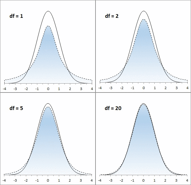
Рис. 1. Нормальная кривая и кривые t-распределения; df – число степеней свободы (от англ. degrees of freedom); gif-файл создан с помощью бесплатного сервиса ezgif.com, на который меня навела Евгения Крюкова
Скачать заметку в формате Word или pdf, примеры в формате Excel
Подход пивовара
В начале XX века Уильяму Сили Госсету, химику и статистику ирландской пивоваренной компании Guinness, потребовалось установить, какой из двух сортов ячменя дает лучшее пиво с большим выходом.[1] Ранее была разработана статистика нормального распределения, позволяющая находить доверительный интервал на основе случайной выборки, состоящей из не менее чем 30 объектов. К сожалению, у Госсета не было возможности протестировать большое число партий пива, изготовленных из каждого сорта ячменя. Однако он не отказался от своей затеи измерить то, что как будто не поддавалось оценке, и решил вывести новый вид распределения для крайне малых выборок. К 1908 г. Госсет разработал новый эффективный метод, который назвал t-статистикой, и захотел опубликовать результаты своей работы.
Однако у Guinness уже были проблемы с разглашением коммерческой тайны, и служащим компании было запрещено публиковать любую информацию о бизнес-процессах. Госсет понимал значение своей работы. Ему сильнее хотелось рассказать о своей идее, чем добиться немедленного признания. Поэтому он опубликовал статью под псевдонимом Стьюдент. И хотя истинный автор давно известен, практически во всех работах по статистике метод называется t-статистикой Стьюдента.
От физических значений к z-статистике
Колоколообразная кривая нормального распределения описывается формулой:
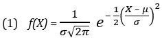
где f(X) – вероятность значения Х; f(X) откладывается по оси ординат; е — основание натурального логарифма; μ — математическое ожидание генеральной совокупности, σ — стандартное отклонение генеральной совокупности, X — произвольное значение непрерывной случайной величины; X откладывается по оси абсцисс; –∞ < X < +∞ (о вычислении μ и σ подробнее см. Определение среднего значения, вариации и формы распределения. Описательные статистики).
Формула (1) довольно сложная, и в докомпьютерную эру статистики использовали заранее рассчитанные таблицы. Поскольку составление таблиц для всего разнообразия Х, μ и σ дело неподъемное, была придумана стандартизация, которая состоит в приведении физических величин к z-единицам, путем простой арифметической подстановки

В этом случае всё многообразие нормальных кривых сводится к единому стандартизованному распределению:
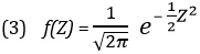
где математическое ожидание (среднее) стандартизованного нормального распределения μ = 0, а стандартное отклонение σ = 1. Фактически, z – это десятичное число, для которого σ = 1, μ = 0.
Сейчас функция в Excel НОРМ.РАСП(x;среднее;стандартное_откл;интегральная) значительно упростила работу с формулой (1). Однако, заложенная традиция сохранилась, и статистики обсуждают особенности распределения, критические границы и т.п. в терминах стандартного нормального распределения (рис. 2). Для последнего в Excel используется функция НОРМ.СТ.РАСП(z;интегральная).
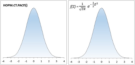
Рис. 2. Формула (3) реализована в Excel с помощью функции НОРМ.СТ.РАСП(); по оси абсцисс – z-единицы, по оси ординат – вероятность.
Для перехода от стандартного распределения к физическим величинам нужно применить обратное преобразование:
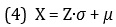
Допустим вы изучаете время загрузки некой Web-страницы, и выясняете, что оно распределено нормально, причем математическое ожидание равно μ = 7с, а стандартное отклонение σ = 2с. Как показывает рис. 3, каждому значению переменной X соответствует нормированное значение Z, полученное с помощью формулы преобразования (2). Следовательно, время загрузки, равное 9с, на одну стандартную единицу превышает математическое ожидание: Z = (9 – 7) / 2 = +1, а время загрузки равное 1с на три z-единицы (стандартных отклонения) меньше математического ожидания: Z = (1 – 7) / 2 = –3.
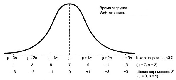
Рис. 3. Преобразование физических значений в z-значения для μ = 7, σ = 2
Описанные выше z-единицы используют для индивидуальных оценок, т.е. для измерений, приписываемых отдельным элементам выборки (например, рост каждого ученика школы). Если в качестве точек кривой нормального распределения берутся средние значения выборок (например, средний рост учеников различных классов), используют термин z-значение или z-статистика:[2]
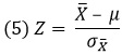
где X̅ – среднее значение выборки (средний рост учеников 5А класса), μ – среднее значение генеральной совокупности (средний рост всех учеников школы),  – стандартная ошибка средних (стандартное отклонение среднего роста учеников отдельных классов от среднего роста всех учеников школы). Последняя рассчитывается по формуле:

где σ – стандартная ошибка индивидуальных значений, n – размер выборки (число учеников в классе).
t-значение
Допустим, вы предполагаете, что дизельные двигатели автомобилей определенной модели выбрасывают в атмосферу больше оксида азота, чем заявлено в рекламных объявлениях. Вы знаете, что стандарт устанавливает ограничение на выбросы – не более 0,4 грамма на милю пробега. Вы хотели бы сравнить эмпирически полученные результаты не со средним по генеральной совокупности, а с этим стандартом – 0,4 г/милю. Это целевое значение, а не параметр генеральной совокупности. Вы тестируете пять автомобилей данной модели и измеряете уровень выброса оксида азота в дорожных условиях. Далее вы вычисляете среднее количество выбросов оксида азота для пяти автомобилей и находите стандартное отклонение. Наконец, вы находите величину:
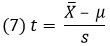
где X̅ – средний уровень выбросов диоксида азота для пяти автомобилей; μ = 0,4 – установленный стандартом граничный уровень выбросов оксида азота;[3] s — стандартное отклонение уровня выбросов оксида азота по результатам для пяти автомобилей.
Это отношение очень похоже на формулу (2) для z-значения, но в действительности это t-значение. z- и t-значения отличаются тем, что для нахождения t-значения используется стандартное отклонение, полученное на основе выборочных результатов s, а не известное значение параметра генеральной совокупности σ. Использование латинской буквы s вместо греческой буквы σ для обозначения стандартного отклонения напоминает о том, что в данном случае значение стандартного отклонения является выборочной оценкой (статистикой), а не известным параметром.
Плотность распределения t-значений рассчитывается не с помощью формулы (3), а существенно сложнее. Я не привожу её здесь, поскольку сейчас в лоб ее никто не считает. Все используют готовые функции в статистических пакетах.
В Excel есть ряд функций, работающих с t-статистикой (рис. 4). Функции, имена которых включают часть РАСП, принимают t-значение в качестве аргумента и возвращают вероятность. Функции, имена которых включают часть ОБР, принимают значение вероятности в качестве аргумента и возвращают t-значение. Две последние функции на рис. 4 устарели и оставлены для обратной совместимости с более ранними версиями Excel.
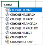
Рис. 4. Семейство функций в Excel, работающих с t-статистикой Стьюдента
Степени свободы
Кривая t-распределения аналогична стандартной нормальной кривой, но ее форма немного меняется в зависимости от количества наблюдений, использованных для ее построения. В общем случае количество степеней свободы df = n – k, где n — количество наблюдений в выборке, а k — количество статистик, фиксированных для выборки. Например, если мы просто изучаем выборку, то k = 1, так как мы зафиксировали только среднее значение выборки. Если мы изучаем регрессионную зависимость от одной переменной, то k = 2; зафиксированы две статистики: среднее по выборке и наклон регрессионной кривой. Каждая дополнительная независимая переменная в регрессионной зависимости уменьшает число степеней свободы на единицу.
Во все функции Excel, предназначенные для работы с t-распределением, вторым аргументом входит количество степеней свободы df. Этот параметр необходим Excel для того, чтобы правильно вычислить форму кривой плотности t-распределения и вернуть корректное значение вероятности t-значения, заданного с помощью первого аргумента. Так для одного и того же z-значения = t-значению = 2,5 вероятность встретить его зависит от размера выборки (числа степеней свободы; рис. 5).
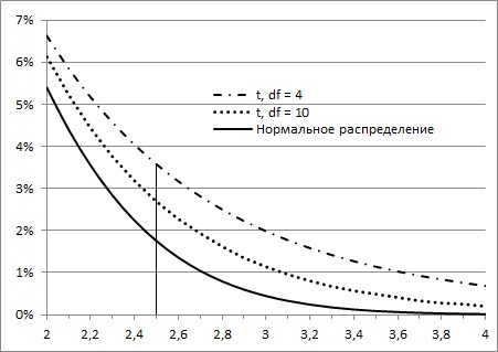
Рис. 5. Вероятность появления z- или t-значения зависит от того, какое распределение используется
То, насколько толстыми или тяжелыми являются хвосты t-распределения можно выразить количественно (рис. 6). Так, например, в пределах одного стандартного отклонение от среднего при нормальном распределении находится 68,27% значений. Для t-распределения с двумя степенями свободы такая вероятность существенно меньше – 57,74%.
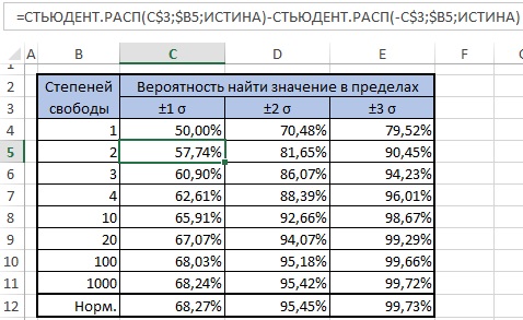
Рис. 6. Сравнение нормального и t-распределений
Функции Excel для работы с t-распределением
Рассмотрим работу функций Excel подробнее. Функция =СТЬЮДЕНТ.РАСП(t-значение;df;интегральная) возвращает левостороннее t-распределение Стьюдента (рис. 7). t-значение должно быть стандартизовано согласно формуле (7), т.е., выражено в долях стандартного отклонения σ при математическом ожидание генеральной совокупности µ = 0. Последний аргумент функции СТЬЮДЕНТ.РАСП() является логическим значением. Если он равен ЛОЖЬ, возвращается функция плотности распределения, т.е., вероятность для одного t-значения – Р(Х=t). Если он равен ИСТИНА, функция возвращает интегральное (накопленное) значение, т.е., вероятность попасть в интервал от минус бесконечности до t-значения – Р(Х≤t).
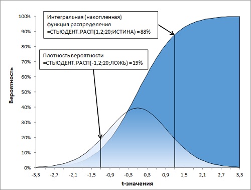
Рис. 7. Левостороннее t-распределение Стьюдента, функция Excel СТЬЮДЕНТ.РАСП()
Если функцию СТЬЮДЕНТ.РАСП() дополнить простыми арифметическими действиями, можно решить множество задач, связанных с t-распределением. Некоторые из них представлены ниже (рис. 8; во всех случаях df = 20):
- какова вероятность найти значение за пределами диапазона ±2,4σ от среднего значения Р(|Х|≥2,4)? =СТЬЮДЕНТ.РАСП(-2,4;20;ИСТИНА)*2
- какова вероятность найти значение внутри диапазона ±1,8σ от среднего значения Р(|Х|≤1,8)? =СТЬЮДЕНТ.РАСП(1,8;20;ИСТИНА)-СТЬЮДЕНТ.РАСП(-1,8;20;ИСТИНА) или, учитывая симметричность t-распределения, =(0,5-СТЬЮДЕНТ.РАСП(-1,8;20;ИСТИНА))*2
- какова вероятность найти значение справа от 2σ Р(Х≥2)?
=1-СТЬЮДЕНТ.РАСП(2;20;ИСТИНА) - какова вероятность среднего значения Р(Х=0)?
=СТЬЮДЕНТ.РАСП(0;20;ЛОЖЬ)
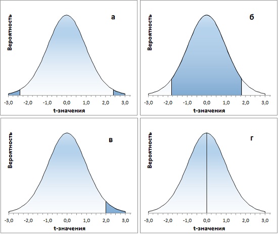
Рис. 8. Функция Excel СТЬЮДЕНТ.РАСП() позволяет решать основные задачи с t-распределением
Функция СТЬЮДЕНТ.РАСП.ПХ() возвращает правостороннее t-распределение, причем только интегральное. Т.е., она показывает накопленную вероятность, начиная с правой точки +∞ при движении влево – Р(X≥t).[4] У функции только два аргумента: t-значение и число степеней свободы. Она чуть более удобна, чем СТЬЮДЕНТ.РАСП() в задачах, где нас интересует вероятность обнаружить то или иное значение правого хвоста. Для примера (в) выше (см. также рис. 8в) формула будет такой: =СТЬЮДЕНТ.РАСП.ПХ(2;20).
Функция СТЬЮДЕНТ.РАСП.2Х() возвращает двустороннее t-распределение Стьюдента – P(|X|≥t) или P(X≥t или X≤-t). Как и функция СТЬЮДЕНТ.РАСП.ПХ(), она имеет два аргумента (t-значение и число степеней свободы), и возвращает только интегральное значение. Функция СТЬЮДЕНТ.РАСП.2Х() показывает накопленную вероятность для двух симметричных хвостов. Она чуть более удобна, чем СТЬЮДЕНТ.РАСП() в задачах, где нас интересует вероятность обнаружить два хвоста сразу. При этом задать нужно t-значение правого хвоста (отрицательные t-значения функция не принимает). Для примера (а) выше (см. также рис. 9а) формула будет такой: =СТЬЮДЕНТ.РАСП.2Х(2,4;20).
t-критерий
Одно из важных применений t-статистики связано с ответом на вопрос, насколько выборка характерна для генеральной совокупности? Например, если в генеральной совокупности среднее μ, а в выборке – х̅, какова вероятность, что выборка сделана из этой генеральной совокупности, а не из другой?
Рассмотрим пример (рис. 9). Исследуется зависимость веса от роста. Функция массива ЛИНЕЙН() (ячейки D2:E6), возвращает, в частности, наклон регрессионной кривой, он же коэффициент регрессии (ячейка D2) и стандартную ошибку коэффициента регрессии (ячейка D3). На рис. 9 данные роста и веса помещены на точечную диаграмму. На ней изображена регрессионная прямая (пунктирная линия; чтобы вывести ее, кликните в области диаграммы правой кнопкой мыши, и выберите опцию Добавить линию тренда…). Выведена также и формула регрессионной кривой y = 2,0922x – 3,5905 (естественно, коэффициент при х равен значению в ячейке D2).
t-критерий параметра = значение параметра, деленное на стандартную ошибку параметра
В нашем случае t-критерий коэффициента регрессии = коэффициент регрессии / стандартная ошибка коэффициента регрессии = 2,0922 / 0,8177 = 2,559 (ячейка Е8).
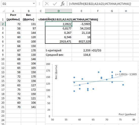
Рис. 9. Коэффициент регрессии = 2,0922 и t-критерий коэффициента регрессии = 2,559
Допустим, в генеральной совокупности вес не зависит от роста (нулевая гипотеза; на рис. 9 изображена сплошной прямой). Это значит, что коэффициент регрессии генеральной совокупности равен 0. В нашей выборке из 20 человек, мы обнаружили линейную зависимость веса от роста с коэффициентом регрессии (коэффициентом при х) = 2,0922. Если нормировать эту величину на стандартную ошибку, мы получим безразмерную величину = 2,559. Т.е., подсчитанный нами коэффициент регрессии в выборке на 2,559 сигм отстоит от нуля.
Насколько невероятно (или вероятно) получить такое отклонение в выборке, если в генеральной совокупности коэффициент регрессии = 0? Можно ли дать определение того, какое событие можно считать «невероятным». Считать ли его таковым, если оно происходит один раз в серии из 20 испытаний? Или в серии из 100 испытаний? А может быть, из 1000 испытаний? Как правило, событие считают «невероятным», если оно может произойти не чаще, чем в одном случае из двадцати.
Итак, в качестве нулевой гипотезы можно принять, что вес не зависит от роста. В качестве альтернативной гипотезы мы предположим, что вес положительно коррелирован с ростом (чем больше рост, тем больше вес). Мы отклоним нулевую гипотезу, только если t-значение коэффициента регрессии попадет в правый хвост распределения в область, соответствующую 5% всей площади под кривой (α = 0,05). Это, как раз, произойдет не чаше, чем один раз на двадцать выборок (рис. 10).
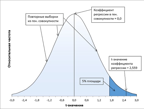
Рис. 10. Расположение t-значения коэффициента регрессии (2,559) на кривой t-распределения Стьюдента (df = 18) показывает, что его вероятность около 1% не превышает α-уровень = 5%. Нулевая гипотеза может быть отвергнута. Статистики выборки говорят о зависимости веса от роста.
Расчет t-значения, соответствующего заданному уровню значимости
Проблема выбора «уровня невероятности», т.е. уровня статистической значимости, или α-уровня, десятилетиями будоражила статистиков. Найти ответы на подобные вопросы зачастую очень трудно, и многие исследователи лишь пожимают плечами и выбирают для альфа-уровня одно из общепринятых значений: р < 0,05 или р < 0,01. Почему именно такие значения?
Главная причина — это то, что в течение многих лет исследователи должны были полагаться на справочные таблицы, позволяющие найти такое t-значение, которое можно было бы считать «статистически значимым» на уровне 0,05 или 0,01 (таблиц для других α-значений практически не было). В наше время определение критического значения t-статистики при любом заданном уровне значимости не составляет труда.
В Excel есть две функции для расчета t-критерия по уровню значимости (вероятности). СТЬЮДЕНТ.ОБР(вероятность;степени_свободы) возвращает левостороннее обратное t-распределение. В качестве первого аргумента функция принимает накопленную вероятность, начиная с –∞. Как правило, используется для односторонних тестов. В случае использования в двустороннем тесте α-значение следует разделить на 2. Например, t-значение для 5%-ного уровня значимости на рис. 10 можно найти с помощью формул =–СТЬЮДЕНТ.ОБР(0,05;18) или =СТЬЮДЕНТ.ОБР(1–0,05;18). В обоих случаях ответ 1,7341. В первом случае СТЬЮДЕНТ.ОБР(0,05;18) возвращает значение –1,7341, соответствующее 5%, накопленным от –∞ до –1,7341 (рис. 11а). Для получения окончательного ответа нужно воспользоваться свойством симметрии кривой распределения, и добавить знак минус перед функцией. Во втором случае СТЬЮДЕНТ.ОБР(1–0,05;18) возвращает значение 1,7341, соответствующее 95%, накопленным от –∞ до 1,7341 (рис. 11б).
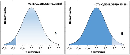
Рис. 11. Односторонний t-критерий с уровнем значимости α = 5%
Вторая функция =СТЬЮДЕНТ.ОБР.2Х() используется в двусторонних тестах, когда мы допускаем, что исследуемое значение может отклоняться в обе стороны от среднего. В формулу следует подставить α-уровень значимости, функция сама разобьет его на две части и вернет значение, соответствующее двум симметричным хвостам (рис. 12; сравните с рис. 11а).
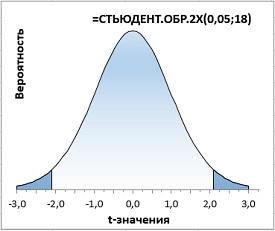
Рис. 12. Двусторонний t-критерий с уровнем значимости α = 5%
Ошибка первого рода
Предположим, перед вами стоит задача увеличить трафик нескольких веб-сайтов. Вы договариваетесь с владельцем популярного рекламного сайта о том, чтобы на его страницах отображались ссылки на 16 сайтов, случайным образом выбираемых из списка сайтов, контролируемых вашей компанией. Другие ваши 16 сайтов, также выбираемые случайным образом, не будут продвигаться в течение месяца.
Вы намереваетесь сравнить между собой средние показатели посещений сайтов, ссылки на которые специально продвигаются поставщиком рекламных услуг, и остальных сайтов. Вы останавливаете свой выбор на направленной гипотезе с альфа-уровнем 0,05: только если специально продвигаемые сайты характеризуются большим средним количеством посещений и только если различие между двумя группами сайтов настолько велико, что при многократном повторении данного испытания оно может случайно встретиться не чаще, чем в одном случае из 20, вы будете отбрасывать гипотезу о том, что специальное продвижение сайта не влияет на среднее количество его посещений.
Через месяц вы получаете свои данные и обнаруживаете, что средний показатель для вашей контрольной группы – сайтов, не получающих специального продвижения, – составляет 45 посещений в час, а для продвигаемых сайтов – 55 посещений в час. Стандартная ошибка среднего равна 5.
Итак, у нас имеется контрольная группа из 16 сайтов (df = 15), правосторонний однонаправленный тест с α-уровнем = 0,05. t-значение определяется по формуле =-СТЬЮДЕНТ.ОБР(0,05;15) и равно 1,7531. Критическое значение посещаемости определяется по формуле (4) и равно: t-значение * стандартное отклонение выборки + среднее по выборке = 1,7531 * 5 + 45 = 53,8. Среднее по экспериментальной группе (55) больше критического t-значения (55 > 53,8). Мы можем отвергнуть нулевую и принять альтернативную гипотезу – продвижение сайтов влияет на посещаемость (рис. 13).
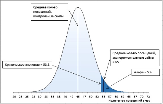
Рис. 13. Попадание среднего значения внутрь α-уровня позволяет отвергнуть нулевую гипотезу
Но, значение альфа-уровня полностью контролируется нами — это наше правило принятия решений. Если бы мы установили для альфа-уровня значение 0,01, мы бы не отвергли нулевую гипотезу (рис. 14). Мы могли бы сказать, что среднее экспериментальной группы происходит из той же генеральной совокупности, что и среднее контрольной группы. Итак, статистическая ошибка I рода: мы отвергаем нулевую гипотезу, когда она верна.
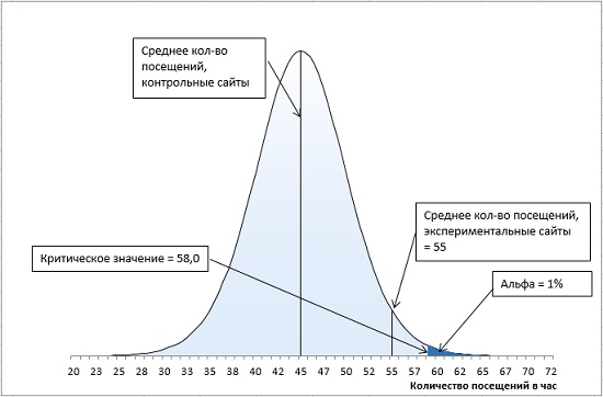
Рис. 14. Для α-уровня = 0,01 среднее экспериментальной группы не позволяет отвергнуть нулевую гипотезу
Что же мешает установить α-уровень достаточно маленьким, и не отвергать нулевую гипотезу, когда она верна? …Ошибка II рода, заключающаяся в том, что мы не принимаем альтернативную гипотезу, хотя она верна.
Ошибка второго рода
Представьте, что существуют две генеральные совокупности: одна из них состоит из сайтов, не получающих специального продвижения, вторая — из сайтов, получающих продвижение. Если вы повторите свое месячное исследование сотни или даже тысячи раз, то, возможно, получите две колоколообразные кривые (рис. 15).
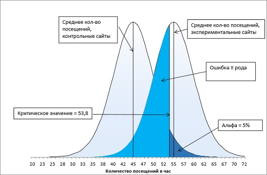
Рис. 15. Ошибка второго рода при α-уровне = 0,05
Иногда среднее значение экспериментальной группы будет происходить из правого хвоста левой кривой распределения исключительно из-за выборочной ошибки. Поскольку в данном случае среднее экспериментальной группы превышает среднее контрольной группы более чем на 1,75 стандартной ошибки (попадает в область α-уровня = 0,05), вы должны отвергнуть нулевую гипотезу, даже если обе генеральные совокупности в действительности имеют одно и то же среднее. Такое неверное отбрасывание нулевой гипотезы, когда в действительности она является истинной, мы назвали ошибкой I рода. В терминах рис. 15 ошибка I рода – приписывание среднего результата экспериментальной выборки, равное 55, правой кривой, а не хвосту левой кривой.
Кривая слева представляет генеральную совокупность веб-сайтов, не получающих специального продвижения. На протяжении месяца частота посещений для некоторых из этих сайтов (очень немногих) составит всего 25 посещений в час, тогда как для других, столь же немногочисленных, – 62 посещения в час. Но 90% всех средних показателей выборок лежат в диапазоне 36,2–53,8 посещений в час.
Кривая справа представляет специально продвигаемые сайты. Как правило, показатели для них примерно на 10 посещений в час выше, чем для сайтов, представленных кривой слева. Их общее среднее составляет 55 посещений в час. Однако большая часть этой информации скрыта от вас. У вас отсутствуют данные о генеральной совокупности, и вы располагаете только результатами двух извлеченных вами выборок, но и этого вам будет вполне достаточно.
Рассмотрим правую кривую на рис. 15. Площадь под этой кривой от минимальных до критического значения (равного 53,8) выделена ярко голубым. Она определяет вероятность ошибки II рода. Средние выборок, проистекающие из этой области, мы относим к левой кривой, а не к правой. Для количественной оценки вероятности ошибки II рода найдем t-значение границы для правой кривой по формуле (7):
Вероятность того, что значение относится к правой кривой и лежит в диапазоне t-значений от –∞ до –0,247 определяется формулой =СТЬЮДЕНТ.РАСП(-0,247;15;ИСТИНА) = 0,404. Т.е., при выбранном нами α-уровне = 0,05 с вероятностью 40,4% мы отклоним альтернативную гипотезу, хотя она верна!
Что произойдет, если мы выберем α-уровень = 0,01, как на рис. 14? Вероятность ошибки II рода увеличится до 72,2% (рис. 16).
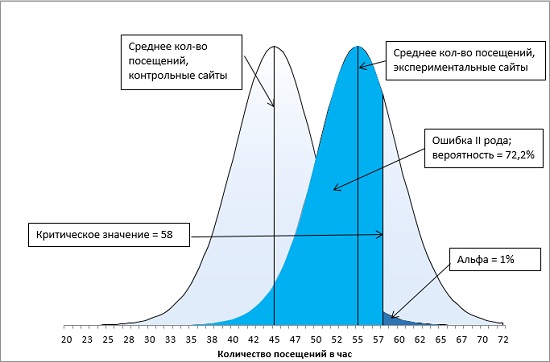
Рис. 16. Ошибка второго рода при α-уровне = 0,01
Статистическая мощность
Вероятность, количественно определяющую величину ошибки второго рода, называют β (на рис. 16 β = 72,2%). А вероятность р = (1 – β) – статистической мощностью (рис. 17).
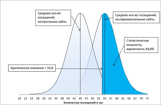
Рис. 17. Статистическая мощность исследования при α-уровне = 0,05
Чем выше статистическая мощность, тем больше вероятность того, что мы отклоним нулевую гипотезу и примем альтернативную гипотезу. На мощность влияют четыре основных фактора:
- Тип теста (переход от двунаправленного теста к однонаправленному увеличивает мощность).
- Уровень α, то есть вероятность ошибки I рода: более высокая α увеличивает мощность.
- Разница между средними значениями выборок (мощность выше при большей разнице).
- Стандартная ошибка среднего (чем ниже ошибка, тем мощность выше).
Давайте на нашем примере рассмотрим, как каждый из указанных факторов изменяет мощность, считая, что факторы меняться по одному (рис 18; расчеты и формулы можно найти в файле Excel).
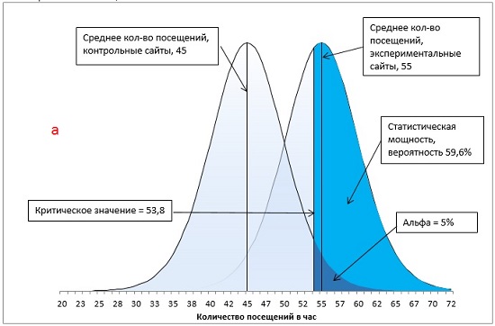
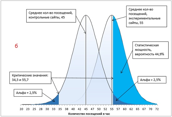

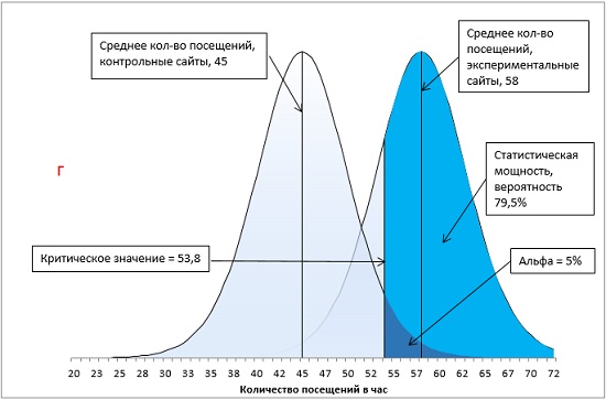
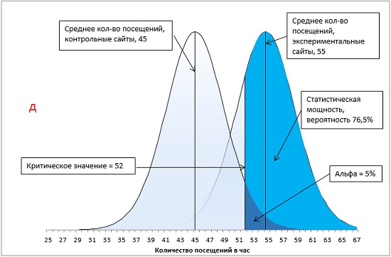
Рис. 18. Методы увеличения статистической мощности: а) базовый вариант; б) ненаправленная гипотеза; в) увеличение α с 0,05 до 0,1; г) увеличение разницы между средними экспериментальной и контрольной групп с 10 до 13 посещений в час; д) увеличение размера групп с 16 до 24 сайтов.
Первый метод повышения статистической мощности связан с подготовкой эксперимента. Если вместо ненаправленной гипотезы (двуххвостовой тест) использовать направленную (однохвостовой тест), вся величина α-уровня отнесется к одному хвосту распределения (сравните рис. 18а и 18б). В результате критическое значение сместится в сторону среднего значения распределения. Чем ближе критическое значение к среднему, тем более вероятно, что вы получите результат, превышающий критическое значение, что увеличивает статистическую мощность тестов. В нашем примере, мощность возрастет с 44,9% до 59,6%.
Второй метод повышения мощности теста предлагает ослабить α-уровень. Например, увеличивая α от 0,05 до 0,10, вы увеличиваете вероятность совершения ошибки I рода, но уменьшаете вероятность совершения ошибки II рода (сравните рис. 18а и 18в). В нашем примере, мощность возросла с 59,6% до 74%.
Оставшиеся два метода повышения статистической мощности основаны на формуле расчета t-статистики:

где t – t-значение для среднего выборки (а не для индивидуального значения), X̅ – среднее значение выборки, μ – среднее значение генеральной совокупности (или среднее значение контрольной выборки), – стандартная ошибка средних по выборкам (а не индивидуальных значений), равная:
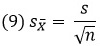
где s – стандартная ошибка индивидуальных значений, n – размер выборки.
Для увеличения t-статистики (и, как следствие, статистической мощности) нужно, либо увеличить числитель, либо уменьшить знаменатель в формуле (8). Для увеличения разности X̅ – μ требуется внесение изменений в проведение эксперимента. Как это сделать, непростой вопрос, решаемый в каждом конкретном случае. В нашем примере, увеличение X̅ с 55 до 58 посещений в час при неизменном μ = 45, приведет к росту статистической мощности с 59,6% до 79,5% (рис. 18г).
И, наконец, уменьшение величины знаменателя тестовой статистики в формуле (8), есть не что иное, как уменьшение стандартной ошибки . Одним из способов уменьшения стандартной ошибки является увеличение размера выборки, n. В соответствии с формулой (9), чем больше n, тем меньше . В нашем примере, при неизменной стандартной ошибке индивидуальных значений s, увеличение контрольной и экспериментальной групп с 16 до 24 сайтов приведет к уменьшению с 5 до 4,1 и росту мощности с 59,6% до 76,5% (рис. 18д).
Один из хороших способов познакомиться с влиянием разных факторов на мощность – это поэкспериментировать с графическим калькулятором мощности, например, здесь.
Основные положения заметки
t-статистика Стьюдента используется вместо нормального распределения: а) для малых выборок; б) если стандартное отклонение генеральной совокупности σ не известно.
t-распределение представлено семейством распределений; дополнительный параметр – размер выборки или число степеней свободы.
Число степеней свободы равно размеру выборки минус число фиксированных статистик выборки (среднее, коэффициент регрессии, …)
Чем больше степеней свободы, тем ближе t-распределение к нормальному.
Функции в Excel, имена которых включают часть РАСП, принимают t-значение в качестве аргумента и возвращают вероятность. Функции, имена которых включают часть ОБР, принимают значение вероятности в качестве аргумента и возвращают t-значение.
Для подстановки в функции Excel значения предварительно должны быть стандартизованы.
Ошибка I рода: отбрасывание нулевой гипотезы, когда в действительности она является истинной. Ошибка II рода: не принятие альтернативной гипотезы, хотя она верна. Чем больше ошибка первого рода, тем меньше ошибка второго рода.
Критерий отнесения события к маловероятному является произвольным. Традиционно маловероятным считают событие, происходящее не чаще, чем 1 раз из 20 попыток.
Один из основных методов уменьшения ошибки второго рода – увеличение элементов в выборке.
[1] При написании замети использованы материалы книг: Дуглас Хаббард. Как измерить всё, что угодно, Левин и др. Статистика для менеджеров, Сара Бослаф. Статистика для всех, Конрад Карлберг. Регрессионный анализ в Microsoft Excel.
[2] На самом деле, можно встретить довольно много различных терминов в отношении нормированных значений z. Ориентируйтесь не на названия, а на суть понятий.
[3] Могут высказать справедливое замечание, что не следует обозначать граничный уровень так же, как и математическое ожидание генеральной совокупности µ. Соглашусь, но всё же использую обозначение, поскольку, в иных задачах здесь часто фигурирует именно математическое ожидание генеральной совокупности µ.
[4] Некоторые авторы указывают знак меньше или равно для левостороннего распределения Р(Х≤t), и больше для правостороннего Р(X>t). Однако, для t=0 значения СТЬЮДЕНТ.РАСП(0;df;ИСТИНА) = СТЬЮДЕНТ.РАСП.ПХ(0;df) = 0,5 для любого значения df. На мой взгляд, Excel при интегральном расчете трактует границу, как исчезающе малую. Поэтому, нет разницы, использовать знак ≥ или >.