Средняя ошибка
полученная как среднеарифметическое
из истинных ошибок, дает неверное
представление о точности результатов,
так как при сложении положительных и
отрицательных ошибок компенсируется.
Поэтому определяют среднее арифметическое
из абсолютных значений ошибок.
v=[|∆|]/n,
где ∆-среднеарифметическое, n-число
измерений.
В таком случае
средняя ошибка наиболее достоверна, но
средняя ошибка недостаточно точно
характеризует результаты измерений,
т.к сглаживает влияние больших по
величине ошибок.
Чтобы усилить их
влияние нужно их возвести в квадрат и
получают средние
квадратические ошибки.
m=√([∆2]/n)
Преимущество СКО
по сравнению со средними:
1.Учитывают влияние
больших по величине ошибок.
2.СКО одного измерения
(me)
определенная из небольшого числа
измерений мало отличается от СКО большого
числа таких же измерений.
При оценке точности
результатов измерений достаточно чтобы
в оценке участвовали 4 рез-та, которые
дадут однозначное значение ошибки.
При оценке точности
после определения СКО необходимо
вычислить ошибку самой ошибки (надежность
ошибки):
mml=ml/√2n
Зная СКО можно
установить предельную ошибку, абсолютное
значение которой является верхней
границей допустимых при данных условиях
измерений размеров ошибок. ∆пр=ґm,
где ґ=2;2,5;3. Предельная ошибка устанавливается
инструкциями на все виды работ и
называется служебный
допуск.
Вероятная ошибка
— такое значение случайной ошибки при
данных условиях измерения по отношению
к которой ошибки и большие и меньшие по
абсолютной величине встречаются
одинаково часто. В теории вероятности
доказано, что при достаточно большом
числе измерений существуют следующие
зависимости: вероятная ошибка составляет
2/3 квадратической ошибки, а средняя
ошибка составляет 4/5 от средней
квадратической ошибки.
r=2/3m;
v=4/5m.
Истинная, средняя,
вероятная, СКО, предельные ошибки
называются абсолютными.
В тех случаях
когда на точность измерений влияет
размер определяемой величины, то оценка
точности по абсолютной ошибке становится
недостаточной и судить о качестве
измерений нельзя.
Во всех таких
случаях для точности применяют понятие
относительная
ошибка —
отвлеченное число выражающее отношение
абсолютной ошибка измерения к его
результату.
13. Математическая обработка равноточных измерений. Арифметическое среднее, ско арифметической середины.
1.Имеется
ряд равноточных измерений l1,l2…,ln.
За окончательное значение принимаем
среднее из них.
L=(l1+l2+…+ln)/n=[l]/n.
Сравним каждый
результат с точным значением x
и получим ряд истинных ошибок.
∆1=l1-x
∆2=l2-x
…..
∆n=ln-x
где х — точное
значение измеренной величины.
Сложим все и получим
[∆]=[l]-nx.
Выразим отсюда
величину точного значения
x=[l]/n-[∆]/n.
При бесконечном
числе измерений среднее арифметическое
значение их находится ближе всего к
точному их значению х, чем любой из
результатов измерений (l1,l2…ln)
поэтому его называть вероятнейшим
значением измеренной величины.
2.
Если X-точное
значение измеренной величины, а L
-вероятнейшее значение, то М-ошибка
арифметического среднего или вероятнейшее
значение измереной величины.
М= L-x;
Для вывода формулы
определим зависимость между ошибками.
Воспользуемся рядом истинных ошибок:
∆1=l1-x
∆2=l2-x
…..
∆n=ln-x
Сложим равенства
и разделим на n(количество
измерений).
[∆]/n=([l]/n)-x
[∆]/n=L-x
M=[∆]/n
Возведем в квадрат:
M2=(∆12+∆22+…+∆n2+2∆1∆2+2∆1∆3+…+2∆1∆n+…+2∆2∆3+2∆2∆4+…+2∆2∆n+…+2∆n-1∆n)/n2
В числителе этой
формулы удвоенные произведения имеют
разные знаки и при возрастании числа
измерений сумма их стремится к 0 поэтому
отбросив их получим приближенные
равенства.
M2=(∆12+∆22+…+∆n2)/
n2
M2=[∆2]/n2
ml=√([∆2]/n)
M=ml/√n
mL=
ml/√n
– среднеквадратическая ошибка
вероятнейшего значения через СКО
Средняя ошибка
меньше СКО одного измерения.
14-15.Оценка точности
результатов равноточных измерений по
истинным ошибкам. Формулы, порядок
вычислений.
Случайные ошибки
в ряду измерений отличаются одна от
другой на незначительную величину. О
точности измерений можно судить по
значению средней ошибки.
Средняя ошибка,
полученная как среднее арифметическое
из истинных ошибок, дает неверное
представление о точности результатов,
так как при сложении положительных и
отрицательных ошибок компенсируется.
Поэтому определяют среднее арифметическое
из абсолютных значений ошибок.
v=[|∆|]/n,
где ∆-среднеарифметическое, n-число
измерений.
В таком случае
средняя ошибка будет наиболее достоверна,
но средняя ошибка недостаточно точно
характеризует результаты измерений,
так как сглаживает влияние больших по
величине ошибок.
Чтобы усилить их
влияние, их нужно возвести в квадрат. И
получают средние
квадратические ошибки.
ml=√[∆2/n]
При оценке точности
результатов измерений достаточно, чтобы
в этой оценке участвовали всего лишь 4
результата, которые дадут однозначное
значение ошибки. При оценке точности
после после определения СКО необходимо
вычислить ошибку самой ошибки (надежность
ошибки):
mml=ml/√2n
Соседние файлы в предмете [НЕСОРТИРОВАННОЕ]
- #
14.02.20152.46 Mб6Э.doc
- #
- #
- #
- #
- #
- #
- #
- #
- #
- #
In statistics, the mean squared error (MSE)[1] or mean squared deviation (MSD) of an estimator (of a procedure for estimating an unobserved quantity) measures the average of the squares of the errors—that is, the average squared difference between the estimated values and the actual value. MSE is a risk function, corresponding to the expected value of the squared error loss.[2] The fact that MSE is almost always strictly positive (and not zero) is because of randomness or because the estimator does not account for information that could produce a more accurate estimate.[3] In machine learning, specifically empirical risk minimization, MSE may refer to the empirical risk (the average loss on an observed data set), as an estimate of the true MSE (the true risk: the average loss on the actual population distribution).
The MSE is a measure of the quality of an estimator. As it is derived from the square of Euclidean distance, it is always a positive value that decreases as the error approaches zero.
The MSE is the second moment (about the origin) of the error, and thus incorporates both the variance of the estimator (how widely spread the estimates are from one data sample to another) and its bias (how far off the average estimated value is from the true value).[citation needed] For an unbiased estimator, the MSE is the variance of the estimator. Like the variance, MSE has the same units of measurement as the square of the quantity being estimated. In an analogy to standard deviation, taking the square root of MSE yields the root-mean-square error or root-mean-square deviation (RMSE or RMSD), which has the same units as the quantity being estimated; for an unbiased estimator, the RMSE is the square root of the variance, known as the standard error.
Definition and basic properties[edit]
The MSE either assesses the quality of a predictor (i.e., a function mapping arbitrary inputs to a sample of values of some random variable), or of an estimator (i.e., a mathematical function mapping a sample of data to an estimate of a parameter of the population from which the data is sampled). The definition of an MSE differs according to whether one is describing a predictor or an estimator.
Predictor[edit]
If a vector of 


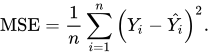
In other words, the MSE is the mean 

In matrix notation,

where 


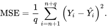
The MSE can also be computed on q data points that were not used in estimating the model, either because they were held back for this purpose, or because these data have been newly obtained. Within this process, known as statistical learning, the MSE is often called the test MSE,[4] and is computed as
Estimator[edit]
The MSE of an estimator 

![{displaystyle operatorname {MSE} ({hat {theta }})=operatorname {E} _{theta }left[({hat {theta }}-theta )^{2}right].}](https://wikimedia.org/api/rest_v1/media/math/render/svg/9a0e1b3bac58f9ba2d2f4ff8b85b2e35a8f4bf78)
This definition depends on the unknown parameter, but the MSE is a priori a property of an estimator. The MSE could be a function of unknown parameters, in which case any estimator of the MSE based on estimates of these parameters would be a function of the data (and thus a random variable). If the estimator
The MSE can be written as the sum of the variance of the estimator and the squared bias of the estimator, providing a useful way to calculate the MSE and implying that in the case of unbiased estimators, the MSE and variance are equivalent.[5]

Proof of variance and bias relationship[edit]
![{displaystyle {begin{aligned}operatorname {MSE} ({hat {theta }})&=operatorname {E} _{theta }left[({hat {theta }}-theta )^{2}right]\&=operatorname {E} _{theta }left[left({hat {theta }}-operatorname {E} _{theta }[{hat {theta }}]+operatorname {E} _{theta }[{hat {theta }}]-theta right)^{2}right]\&=operatorname {E} _{theta }left[left({hat {theta }}-operatorname {E} _{theta }[{hat {theta }}]right)^{2}+2left({hat {theta }}-operatorname {E} _{theta }[{hat {theta }}]right)left(operatorname {E} _{theta }[{hat {theta }}]-theta right)+left(operatorname {E} _{theta }[{hat {theta }}]-theta right)^{2}right]\&=operatorname {E} _{theta }left[left({hat {theta }}-operatorname {E} _{theta }[{hat {theta }}]right)^{2}right]+operatorname {E} _{theta }left[2left({hat {theta }}-operatorname {E} _{theta }[{hat {theta }}]right)left(operatorname {E} _{theta }[{hat {theta }}]-theta right)right]+operatorname {E} _{theta }left[left(operatorname {E} _{theta }[{hat {theta }}]-theta right)^{2}right]\&=operatorname {E} _{theta }left[left({hat {theta }}-operatorname {E} _{theta }[{hat {theta }}]right)^{2}right]+2left(operatorname {E} _{theta }[{hat {theta }}]-theta right)operatorname {E} _{theta }left[{hat {theta }}-operatorname {E} _{theta }[{hat {theta }}]right]+left(operatorname {E} _{theta }[{hat {theta }}]-theta right)^{2}&&operatorname {E} _{theta }[{hat {theta }}]-theta ={text{const.}}\&=operatorname {E} _{theta }left[left({hat {theta }}-operatorname {E} _{theta }[{hat {theta }}]right)^{2}right]+2left(operatorname {E} _{theta }[{hat {theta }}]-theta right)left(operatorname {E} _{theta }[{hat {theta }}]-operatorname {E} _{theta }[{hat {theta }}]right)+left(operatorname {E} _{theta }[{hat {theta }}]-theta right)^{2}&&operatorname {E} _{theta }[{hat {theta }}]={text{const.}}\&=operatorname {E} _{theta }left[left({hat {theta }}-operatorname {E} _{theta }[{hat {theta }}]right)^{2}right]+left(operatorname {E} _{theta }[{hat {theta }}]-theta right)^{2}\&=operatorname {Var} _{theta }({hat {theta }})+operatorname {Bias} _{theta }({hat {theta }},theta )^{2}end{aligned}}}](https://wikimedia.org/api/rest_v1/media/math/render/svg/2ac524a751828f971013e1297a33ca1cc4c38cd6)
An even shorter proof can be achieved using the well-known formula that for a random variable 


![{displaystyle {begin{aligned}operatorname {MSE} ({hat {theta }})&=mathbb {E} [({hat {theta }}-theta )^{2}]\&=operatorname {Var} ({hat {theta }}-theta )+(mathbb {E} [{hat {theta }}-theta ])^{2}\&=operatorname {Var} ({hat {theta }})+operatorname {Bias} ^{2}({hat {theta }})end{aligned}}}](https://wikimedia.org/api/rest_v1/media/math/render/svg/864646cf4426e2b62a3caf9460382eec1a77fe4e)
But in real modeling case, MSE could be described as the addition of model variance, model bias, and irreducible uncertainty (see Bias–variance tradeoff). According to the relationship, the MSE of the estimators could be simply used for the efficiency comparison, which includes the information of estimator variance and bias. This is called MSE criterion.
In regression[edit]
In regression analysis, plotting is a more natural way to view the overall trend of the whole data. The mean of the distance from each point to the predicted regression model can be calculated, and shown as the mean squared error. The squaring is critical to reduce the complexity with negative signs. To minimize MSE, the model could be more accurate, which would mean the model is closer to actual data. One example of a linear regression using this method is the least squares method—which evaluates appropriateness of linear regression model to model bivariate dataset,[6] but whose limitation is related to known distribution of the data.
The term mean squared error is sometimes used to refer to the unbiased estimate of error variance: the residual sum of squares divided by the number of degrees of freedom. This definition for a known, computed quantity differs from the above definition for the computed MSE of a predictor, in that a different denominator is used. The denominator is the sample size reduced by the number of model parameters estimated from the same data, (n−p) for p regressors or (n−p−1) if an intercept is used (see errors and residuals in statistics for more details).[7] Although the MSE (as defined in this article) is not an unbiased estimator of the error variance, it is consistent, given the consistency of the predictor.
In regression analysis, «mean squared error», often referred to as mean squared prediction error or «out-of-sample mean squared error», can also refer to the mean value of the squared deviations of the predictions from the true values, over an out-of-sample test space, generated by a model estimated over a particular sample space. This also is a known, computed quantity, and it varies by sample and by out-of-sample test space.
Examples[edit]
Mean[edit]
Suppose we have a random sample of size 

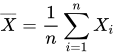
which has an expected value equal to the true mean
![{displaystyle operatorname {MSE} left({overline {X}}right)=operatorname {E} left[left({overline {X}}-mu right)^{2}right]=left({frac {sigma }{sqrt {n}}}right)^{2}={frac {sigma ^{2}}{n}}}](https://wikimedia.org/api/rest_v1/media/math/render/svg/b4647a2cc4c8f9a4c90b628faad2dcf80c4aae84)
where 
For a Gaussian distribution, this is the best unbiased estimator (i.e., one with the lowest MSE among all unbiased estimators), but not, say, for a uniform distribution.
Variance[edit]
The usual estimator for the variance is the corrected sample variance:

This is unbiased (its expected value is

where 
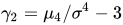
However, one can use other estimators for 

then we calculate:
![{displaystyle {begin{aligned}operatorname {MSE} (S_{a}^{2})&=operatorname {E} left[left({frac {n-1}{a}}S_{n-1}^{2}-sigma ^{2}right)^{2}right]\&=operatorname {E} left[{frac {(n-1)^{2}}{a^{2}}}S_{n-1}^{4}-2left({frac {n-1}{a}}S_{n-1}^{2}right)sigma ^{2}+sigma ^{4}right]\&={frac {(n-1)^{2}}{a^{2}}}operatorname {E} left[S_{n-1}^{4}right]-2left({frac {n-1}{a}}right)operatorname {E} left[S_{n-1}^{2}right]sigma ^{2}+sigma ^{4}\&={frac {(n-1)^{2}}{a^{2}}}operatorname {E} left[S_{n-1}^{4}right]-2left({frac {n-1}{a}}right)sigma ^{4}+sigma ^{4}&&operatorname {E} left[S_{n-1}^{2}right]=sigma ^{2}\&={frac {(n-1)^{2}}{a^{2}}}left({frac {gamma _{2}}{n}}+{frac {n+1}{n-1}}right)sigma ^{4}-2left({frac {n-1}{a}}right)sigma ^{4}+sigma ^{4}&&operatorname {E} left[S_{n-1}^{4}right]=operatorname {MSE} (S_{n-1}^{2})+sigma ^{4}\&={frac {n-1}{na^{2}}}left((n-1)gamma _{2}+n^{2}+nright)sigma ^{4}-2left({frac {n-1}{a}}right)sigma ^{4}+sigma ^{4}end{aligned}}}](https://wikimedia.org/api/rest_v1/media/math/render/svg/cf22322412b8454c706d78671e5d94208675a6e0)
This is minimized when

For a Gaussian distribution, where 


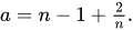
Further, while the corrected sample variance is the best unbiased estimator (minimum mean squared error among unbiased estimators) of variance for Gaussian distributions, if the distribution is not Gaussian, then even among unbiased estimators, the best unbiased estimator of the variance may not be 
Gaussian distribution[edit]
The following table gives several estimators of the true parameters of the population, μ and σ2, for the Gaussian case.[9]
| True value | Estimator | Mean squared error |
|---|---|---|
 |
= the unbiased estimator of the population mean, 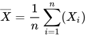 |

|
 |
= the unbiased estimator of the population variance, 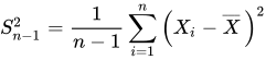 |

|
|
= the biased estimator of the population variance, 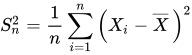 |

|
|
= the biased estimator of the population variance, 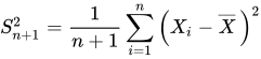 |

|
Interpretation[edit]
An MSE of zero, meaning that the estimator
Values of MSE may be used for comparative purposes. Two or more statistical models may be compared using their MSEs—as a measure of how well they explain a given set of observations: An unbiased estimator (estimated from a statistical model) with the smallest variance among all unbiased estimators is the best unbiased estimator or MVUE (Minimum-Variance Unbiased Estimator).
Both analysis of variance and linear regression techniques estimate the MSE as part of the analysis and use the estimated MSE to determine the statistical significance of the factors or predictors under study. The goal of experimental design is to construct experiments in such a way that when the observations are analyzed, the MSE is close to zero relative to the magnitude of at least one of the estimated treatment effects.
In one-way analysis of variance, MSE can be calculated by the division of the sum of squared errors and the degree of freedom. Also, the f-value is the ratio of the mean squared treatment and the MSE.
MSE is also used in several stepwise regression techniques as part of the determination as to how many predictors from a candidate set to include in a model for a given set of observations.
Applications[edit]
- Minimizing MSE is a key criterion in selecting estimators: see minimum mean-square error. Among unbiased estimators, minimizing the MSE is equivalent to minimizing the variance, and the estimator that does this is the minimum variance unbiased estimator. However, a biased estimator may have lower MSE; see estimator bias.
- In statistical modelling the MSE can represent the difference between the actual observations and the observation values predicted by the model. In this context, it is used to determine the extent to which the model fits the data as well as whether removing some explanatory variables is possible without significantly harming the model’s predictive ability.
- In forecasting and prediction, the Brier score is a measure of forecast skill based on MSE.
Loss function[edit]
Squared error loss is one of the most widely used loss functions in statistics[citation needed], though its widespread use stems more from mathematical convenience than considerations of actual loss in applications. Carl Friedrich Gauss, who introduced the use of mean squared error, was aware of its arbitrariness and was in agreement with objections to it on these grounds.[3] The mathematical benefits of mean squared error are particularly evident in its use at analyzing the performance of linear regression, as it allows one to partition the variation in a dataset into variation explained by the model and variation explained by randomness.
Criticism[edit]
The use of mean squared error without question has been criticized by the decision theorist James Berger. Mean squared error is the negative of the expected value of one specific utility function, the quadratic utility function, which may not be the appropriate utility function to use under a given set of circumstances. There are, however, some scenarios where mean squared error can serve as a good approximation to a loss function occurring naturally in an application.[10]
Like variance, mean squared error has the disadvantage of heavily weighting outliers.[11] This is a result of the squaring of each term, which effectively weights large errors more heavily than small ones. This property, undesirable in many applications, has led researchers to use alternatives such as the mean absolute error, or those based on the median.
See also[edit]
- Bias–variance tradeoff
- Hodges’ estimator
- James–Stein estimator
- Mean percentage error
- Mean square quantization error
- Mean square weighted deviation
- Mean squared displacement
- Mean squared prediction error
- Minimum mean square error
- Minimum mean squared error estimator
- Overfitting
- Peak signal-to-noise ratio
Notes[edit]
- ^ This can be proved by Jensen’s inequality as follows. The fourth central moment is an upper bound for the square of variance, so that the least value for their ratio is one, therefore, the least value for the excess kurtosis is −2, achieved, for instance, by a Bernoulli with p=1/2.
References[edit]
- ^ a b «Mean Squared Error (MSE)». www.probabilitycourse.com. Retrieved 2020-09-12.
- ^ Bickel, Peter J.; Doksum, Kjell A. (2015). Mathematical Statistics: Basic Ideas and Selected Topics. Vol. I (Second ed.). p. 20.
If we use quadratic loss, our risk function is called the mean squared error (MSE) …
- ^ a b Lehmann, E. L.; Casella, George (1998). Theory of Point Estimation (2nd ed.). New York: Springer. ISBN 978-0-387-98502-2. MR 1639875.
- ^ Gareth, James; Witten, Daniela; Hastie, Trevor; Tibshirani, Rob (2021). An Introduction to Statistical Learning: with Applications in R. Springer. ISBN 978-1071614174.
- ^ Wackerly, Dennis; Mendenhall, William; Scheaffer, Richard L. (2008). Mathematical Statistics with Applications (7 ed.). Belmont, CA, USA: Thomson Higher Education. ISBN 978-0-495-38508-0.
- ^ A modern introduction to probability and statistics : understanding why and how. Dekking, Michel, 1946-. London: Springer. 2005. ISBN 978-1-85233-896-1. OCLC 262680588.
{{cite book}}: CS1 maint: others (link) - ^ Steel, R.G.D, and Torrie, J. H., Principles and Procedures of Statistics with Special Reference to the Biological Sciences., McGraw Hill, 1960, page 288.
- ^ Mood, A.; Graybill, F.; Boes, D. (1974). Introduction to the Theory of Statistics (3rd ed.). McGraw-Hill. p. 229.
- ^ DeGroot, Morris H. (1980). Probability and Statistics (2nd ed.). Addison-Wesley.
- ^ Berger, James O. (1985). «2.4.2 Certain Standard Loss Functions». Statistical Decision Theory and Bayesian Analysis (2nd ed.). New York: Springer-Verlag. p. 60. ISBN 978-0-387-96098-2. MR 0804611.
- ^ Bermejo, Sergio; Cabestany, Joan (2001). «Oriented principal component analysis for large margin classifiers». Neural Networks. 14 (10): 1447–1461. doi:10.1016/S0893-6080(01)00106-X. PMID 11771723.
In statistics, the mean squared error (MSE)[1] or mean squared deviation (MSD) of an estimator (of a procedure for estimating an unobserved quantity) measures the average of the squares of the errors—that is, the average squared difference between the estimated values and the actual value. MSE is a risk function, corresponding to the expected value of the squared error loss.[2] The fact that MSE is almost always strictly positive (and not zero) is because of randomness or because the estimator does not account for information that could produce a more accurate estimate.[3] In machine learning, specifically empirical risk minimization, MSE may refer to the empirical risk (the average loss on an observed data set), as an estimate of the true MSE (the true risk: the average loss on the actual population distribution).
The MSE is a measure of the quality of an estimator. As it is derived from the square of Euclidean distance, it is always a positive value that decreases as the error approaches zero.
The MSE is the second moment (about the origin) of the error, and thus incorporates both the variance of the estimator (how widely spread the estimates are from one data sample to another) and its bias (how far off the average estimated value is from the true value).[citation needed] For an unbiased estimator, the MSE is the variance of the estimator. Like the variance, MSE has the same units of measurement as the square of the quantity being estimated. In an analogy to standard deviation, taking the square root of MSE yields the root-mean-square error or root-mean-square deviation (RMSE or RMSD), which has the same units as the quantity being estimated; for an unbiased estimator, the RMSE is the square root of the variance, known as the standard error.
Definition and basic properties[edit]
The MSE either assesses the quality of a predictor (i.e., a function mapping arbitrary inputs to a sample of values of some random variable), or of an estimator (i.e., a mathematical function mapping a sample of data to an estimate of a parameter of the population from which the data is sampled). The definition of an MSE differs according to whether one is describing a predictor or an estimator.
Predictor[edit]
If a vector of
In other words, the MSE is the mean
In matrix notation,
where
The MSE can also be computed on q data points that were not used in estimating the model, either because they were held back for this purpose, or because these data have been newly obtained. Within this process, known as statistical learning, the MSE is often called the test MSE,[4] and is computed as
Estimator[edit]
The MSE of an estimator
This definition depends on the unknown parameter, but the MSE is a priori a property of an estimator. The MSE could be a function of unknown parameters, in which case any estimator of the MSE based on estimates of these parameters would be a function of the data (and thus a random variable). If the estimator
The MSE can be written as the sum of the variance of the estimator and the squared bias of the estimator, providing a useful way to calculate the MSE and implying that in the case of unbiased estimators, the MSE and variance are equivalent.[5]
Proof of variance and bias relationship[edit]
An even shorter proof can be achieved using the well-known formula that for a random variable
But in real modeling case, MSE could be described as the addition of model variance, model bias, and irreducible uncertainty (see Bias–variance tradeoff). According to the relationship, the MSE of the estimators could be simply used for the efficiency comparison, which includes the information of estimator variance and bias. This is called MSE criterion.
In regression[edit]
In regression analysis, plotting is a more natural way to view the overall trend of the whole data. The mean of the distance from each point to the predicted regression model can be calculated, and shown as the mean squared error. The squaring is critical to reduce the complexity with negative signs. To minimize MSE, the model could be more accurate, which would mean the model is closer to actual data. One example of a linear regression using this method is the least squares method—which evaluates appropriateness of linear regression model to model bivariate dataset,[6] but whose limitation is related to known distribution of the data.
The term mean squared error is sometimes used to refer to the unbiased estimate of error variance: the residual sum of squares divided by the number of degrees of freedom. This definition for a known, computed quantity differs from the above definition for the computed MSE of a predictor, in that a different denominator is used. The denominator is the sample size reduced by the number of model parameters estimated from the same data, (n−p) for p regressors or (n−p−1) if an intercept is used (see errors and residuals in statistics for more details).[7] Although the MSE (as defined in this article) is not an unbiased estimator of the error variance, it is consistent, given the consistency of the predictor.
In regression analysis, «mean squared error», often referred to as mean squared prediction error or «out-of-sample mean squared error», can also refer to the mean value of the squared deviations of the predictions from the true values, over an out-of-sample test space, generated by a model estimated over a particular sample space. This also is a known, computed quantity, and it varies by sample and by out-of-sample test space.
Examples[edit]
Mean[edit]
Suppose we have a random sample of size
which has an expected value equal to the true mean
where
For a Gaussian distribution, this is the best unbiased estimator (i.e., one with the lowest MSE among all unbiased estimators), but not, say, for a uniform distribution.
Variance[edit]
The usual estimator for the variance is the corrected sample variance:
This is unbiased (its expected value is
where
However, one can use other estimators for
then we calculate:
This is minimized when
For a Gaussian distribution, where
Further, while the corrected sample variance is the best unbiased estimator (minimum mean squared error among unbiased estimators) of variance for Gaussian distributions, if the distribution is not Gaussian, then even among unbiased estimators, the best unbiased estimator of the variance may not be
Gaussian distribution[edit]
The following table gives several estimators of the true parameters of the population, μ and σ2, for the Gaussian case.[9]
| True value | Estimator | Mean squared error |
|---|---|---|
|
= the unbiased estimator of the population mean, |
|
|
= the unbiased estimator of the population variance, |
|
|
= the biased estimator of the population variance, |
|
|
= the biased estimator of the population variance, |
|
Interpretation[edit]
An MSE of zero, meaning that the estimator
Values of MSE may be used for comparative purposes. Two or more statistical models may be compared using their MSEs—as a measure of how well they explain a given set of observations: An unbiased estimator (estimated from a statistical model) with the smallest variance among all unbiased estimators is the best unbiased estimator or MVUE (Minimum-Variance Unbiased Estimator).
Both analysis of variance and linear regression techniques estimate the MSE as part of the analysis and use the estimated MSE to determine the statistical significance of the factors or predictors under study. The goal of experimental design is to construct experiments in such a way that when the observations are analyzed, the MSE is close to zero relative to the magnitude of at least one of the estimated treatment effects.
In one-way analysis of variance, MSE can be calculated by the division of the sum of squared errors and the degree of freedom. Also, the f-value is the ratio of the mean squared treatment and the MSE.
MSE is also used in several stepwise regression techniques as part of the determination as to how many predictors from a candidate set to include in a model for a given set of observations.
Applications[edit]
- Minimizing MSE is a key criterion in selecting estimators: see minimum mean-square error. Among unbiased estimators, minimizing the MSE is equivalent to minimizing the variance, and the estimator that does this is the minimum variance unbiased estimator. However, a biased estimator may have lower MSE; see estimator bias.
- In statistical modelling the MSE can represent the difference between the actual observations and the observation values predicted by the model. In this context, it is used to determine the extent to which the model fits the data as well as whether removing some explanatory variables is possible without significantly harming the model’s predictive ability.
- In forecasting and prediction, the Brier score is a measure of forecast skill based on MSE.
Loss function[edit]
Squared error loss is one of the most widely used loss functions in statistics[citation needed], though its widespread use stems more from mathematical convenience than considerations of actual loss in applications. Carl Friedrich Gauss, who introduced the use of mean squared error, was aware of its arbitrariness and was in agreement with objections to it on these grounds.[3] The mathematical benefits of mean squared error are particularly evident in its use at analyzing the performance of linear regression, as it allows one to partition the variation in a dataset into variation explained by the model and variation explained by randomness.
Criticism[edit]
The use of mean squared error without question has been criticized by the decision theorist James Berger. Mean squared error is the negative of the expected value of one specific utility function, the quadratic utility function, which may not be the appropriate utility function to use under a given set of circumstances. There are, however, some scenarios where mean squared error can serve as a good approximation to a loss function occurring naturally in an application.[10]
Like variance, mean squared error has the disadvantage of heavily weighting outliers.[11] This is a result of the squaring of each term, which effectively weights large errors more heavily than small ones. This property, undesirable in many applications, has led researchers to use alternatives such as the mean absolute error, or those based on the median.
See also[edit]
- Bias–variance tradeoff
- Hodges’ estimator
- James–Stein estimator
- Mean percentage error
- Mean square quantization error
- Mean square weighted deviation
- Mean squared displacement
- Mean squared prediction error
- Minimum mean square error
- Minimum mean squared error estimator
- Overfitting
- Peak signal-to-noise ratio
Notes[edit]
- ^ This can be proved by Jensen’s inequality as follows. The fourth central moment is an upper bound for the square of variance, so that the least value for their ratio is one, therefore, the least value for the excess kurtosis is −2, achieved, for instance, by a Bernoulli with p=1/2.
References[edit]
- ^ a b «Mean Squared Error (MSE)». www.probabilitycourse.com. Retrieved 2020-09-12.
- ^ Bickel, Peter J.; Doksum, Kjell A. (2015). Mathematical Statistics: Basic Ideas and Selected Topics. Vol. I (Second ed.). p. 20.
If we use quadratic loss, our risk function is called the mean squared error (MSE) …
- ^ a b Lehmann, E. L.; Casella, George (1998). Theory of Point Estimation (2nd ed.). New York: Springer. ISBN 978-0-387-98502-2. MR 1639875.
- ^ Gareth, James; Witten, Daniela; Hastie, Trevor; Tibshirani, Rob (2021). An Introduction to Statistical Learning: with Applications in R. Springer. ISBN 978-1071614174.
- ^ Wackerly, Dennis; Mendenhall, William; Scheaffer, Richard L. (2008). Mathematical Statistics with Applications (7 ed.). Belmont, CA, USA: Thomson Higher Education. ISBN 978-0-495-38508-0.
- ^ A modern introduction to probability and statistics : understanding why and how. Dekking, Michel, 1946-. London: Springer. 2005. ISBN 978-1-85233-896-1. OCLC 262680588.
{{cite book}}: CS1 maint: others (link) - ^ Steel, R.G.D, and Torrie, J. H., Principles and Procedures of Statistics with Special Reference to the Biological Sciences., McGraw Hill, 1960, page 288.
- ^ Mood, A.; Graybill, F.; Boes, D. (1974). Introduction to the Theory of Statistics (3rd ed.). McGraw-Hill. p. 229.
- ^ DeGroot, Morris H. (1980). Probability and Statistics (2nd ed.). Addison-Wesley.
- ^ Berger, James O. (1985). «2.4.2 Certain Standard Loss Functions». Statistical Decision Theory and Bayesian Analysis (2nd ed.). New York: Springer-Verlag. p. 60. ISBN 978-0-387-96098-2. MR 0804611.
- ^ Bermejo, Sergio; Cabestany, Joan (2001). «Oriented principal component analysis for large margin classifiers». Neural Networks. 14 (10): 1447–1461. doi:10.1016/S0893-6080(01)00106-X. PMID 11771723.
Среднеквадратичная ошибка (Mean Squared Error) – Среднее арифметическое (Mean) квадратов разностей между предсказанными и реальными значениями Модели (Model) Машинного обучения (ML):

Рассчитывается с помощью формулы, которая будет пояснена в примере ниже:
$$MSE = frac{1}{n} × sum_{i=1}^n (y_i — widetilde{y}_i)^2$$
$$MSEspace{}{–}space{Среднеквадратическая}space{ошибка,}$$
$$nspace{}{–}space{количество}space{наблюдений,}$$
$$y_ispace{}{–}space{фактическая}space{координата}space{наблюдения,}$$
$$widetilde{y}_ispace{}{–}space{предсказанная}space{координата}space{наблюдения,}$$
MSE практически никогда не равен нулю, и происходит это из-за элемента случайности в данных или неучитывания Оценочной функцией (Estimator) всех факторов, которые могли бы улучшить предсказательную способность.
Пример. Исследуем линейную регрессию, изображенную на графике выше, и установим величину среднеквадратической Ошибки (Error). Фактические координаты точек-Наблюдений (Observation) выглядят следующим образом:

Мы имеем дело с Линейной регрессией (Linear Regression), потому уравнение, предсказывающее положение записей, можно представить с помощью формулы:
$$y = M * x + b$$
$$yspace{–}space{значение}space{координаты}space{оси}space{y,}$$
$$Mspace{–}space{уклон}space{прямой}$$
$$xspace{–}space{значение}space{координаты}space{оси}space{x,}$$
$$bspace{–}space{смещение}space{прямой}space{относительно}space{начала}space{координат}$$
Параметры M и b уравнения нам, к счастью, известны в данном обучающем примере, и потому уравнение выглядит следующим образом:
$$y = 0,5252 * x + 17,306$$
Зная координаты реальных записей и уравнение линейной регрессии, мы можем восстановить полные координаты предсказанных наблюдений, обозначенных серыми точками на графике выше. Простой подстановкой значения координаты x в уравнение мы рассчитаем значение координаты ỹ:

Рассчитаем квадрат разницы между Y и Ỹ:

Сумма таких квадратов равна 4 445. Осталось только разделить это число на количество наблюдений (9):
$$MSE = frac{1}{9} × 4445 = 493$$
Само по себе число в такой ситуации становится показательным, когда Дата-сайентист (Data Scientist) предпринимает попытки улучшить предсказательную способность модели и сравнивает MSE каждой итерации, выбирая такое уравнение, что сгенерирует наименьшую погрешность в предсказаниях.
MSE и Scikit-learn
Среднеквадратическую ошибку можно вычислить с помощью SkLearn. Для начала импортируем функцию:
import sklearn
from sklearn.metrics import mean_squared_error
Инициализируем крошечные списки, содержащие реальные и предсказанные координаты y:
y_true = [5, 41, 70, 77, 134, 68, 138, 101, 131]
y_pred = [23, 35, 55, 90, 93, 103, 118, 121, 129]
Инициируем функцию mean_squared_error(), которая рассчитает MSE тем же способом, что и формула выше:
mean_squared_error(y_true, y_pred)
Интересно, что конечный результат на 3 отличается от расчетов с помощью Apple Numbers:
496.0Ноутбук, не требующий дополнительной настройки на момент написания статьи, можно скачать здесь.
Автор оригинальной статьи: @mmoshikoo
Фото: @tobyelliott
Содержание:
Ошибки измерения: Опыт убеждает, что измерения объектов не могут быть произведены абсолютно точно и каждое конкретное измерение дает лишь, как правило, приближенное значение величины явления, истинное значение которой (A) нам неизвестно. Ошибки измерения (
Рассмотрим такие измерения, которые производятся одним наблюдателем, одним и тем же инструментом, в одинаковых условиях, т. е. равноточные измерения.
Различают два вида ошибок измерения:
- систематические ошибки, т. е. такие, которые при данных условиях проведения измерения имеют вполне определенное значение (например, ошибка измерительного прибора);
- случайные — такие, которые являются результатом взаимодействия большого числа незначительных в отдельности факторов и имеют в каждом отдельном случае различные значения.
Задача математической статистики — предусмотреть возможность возникновения систематических ошибок и добиться их ликвидации или сведения к минимуму.
Случайные ошибки измерения обладают рядом свойств: при большом числе измерений крупные ошибки встречаются реже мелких и число положительных ошибок примерно равно числу отрицательных, вследствие чего сумма всех ошибок близка к нулю.
Если ошибки получаются весьма малыми по сравнению с величиной явления, то ими просто пренебрегают или считаются с наибольшей возможной ошибкой, чтобы обезопасить себя от влияния случайной неточности.
В теории ошибок изучаются те ошибки, которые, являясь, с одной стороны, ошибками случайного характера, по своему абсолютному значению настолько велики, что ими пренебречь нельзя, а с другой стороны, для них существует закон, позволяющий установить зависимость между величиной ошибки и вероятностью ее появления. Закон случайных ошибок, полученный Гауссом, состоит в том, что случайные ошибки подчиняются закону нормального распределения.
Средняя ошибка сводного результата измерения
Принимая за действительное значение измеряемой величины при равноточном измерении среднюю арифметическую из всех результатов n измерений, можно охарактеризовать точность одного измерения с помощью средней арифметической из абсолютных величин значений ошибок:
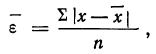
где n — число измерений, х — численное значение отдельных измерений,  — средняя арифметическая из результатов измерений.
За меру точности соответствия принятой средней арифметической  истинному значению измеряемой величины (A) принимают среднюю ошибку сводного результата измерения, вычисляемую по формуле:
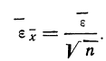
Пример 1. Произведено 10-кратное измерение размера детали (в мм), давшее следующие, расположенные в возрастающем порядке результаты: 138; 139; 140; 141; 141; 142; 142; 143; 144; 145.
Охарактеризуем сначала точность одного измерения, т. е. вычислим среднюю арифметическую из абсолютных значений ошибок. Для этой цели вычислим среднюю арифметическую из результатов измерений:

Найдем ошибки измерения:
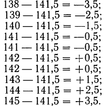
Следовательно:

Теперь можно вычислить среднюю ошибку сводного результата измерения:

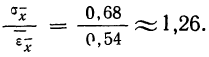
Значит, мерой точности соответствия 141,5 мм истинной величине размера детали является средняя ошибка, равная 0,54 мм.
Средняя квадратическая ошибка
Если в качестве меры точности одного измерения принять не среднюю арифметическую из абсолютных значений ошибок (средняя ошибка), а среднюю квадратическую из ошибок измерений, т. е.
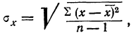
то средняя квадратическая ошибка найденной средней арифметической из ошибок измерения вычисляется по формуле:
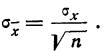
Между средней -квадратической ошибкой и средней ошибкой сводного результата измерения существует связь: 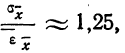 если случайные ошибки подчиняются Гауссову закону нормального распределения.
Пример 2. Используя данные предыдущего примера, находим меру точности одного измерения, т. е. среднюю квадратическую ошибку:

Затем исчисляем среднюю квадратическую ошибку найденной средней арифметической, равной 141,5 мм:

Сопоставляя среднюю квадратическую ошибку сводного результата измерения со средней ошибкой, получаем:
Вероятная ошибка
За меру точности одного измерения иногда принимают вероятную ошибку:

Тогда в качестве вероятной ошибки сводного результата измерения используют соотношение:
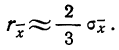
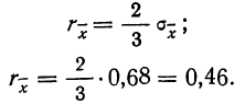
Пример 3. Используя данные предыдущих примеров, находим вероятную ошибку сводного результата измерения:
Наиболее вероятные границы сводных результатов измерения
Математическое ожидание случайной ошибки равно нулю. В качестве значения измеряемой величины применяется средняя арифметическая всех измерений (если они равноточны). Использование отклонений результатов измерений (х) от средней из них  называемых в теории ошибок «кажущимися ошибками»
  позволяет произвести оценку точности соответствия средней арифметической неизвестному истинному значению измеряемой величины (A).
Для этой цели используют удвоенную или утроенную среднюю квадратическую ошибку сводного результата измерения или его вероятную ошибку и получают:

Найденные границы неизвестной истинной величины в случае, если ошибки подчинены нормальному закону распределения Гаусса (чаще всего так и бывает), соблюдаются с большой вероятностью (0,997 и 0,954).
Пример 4. По данным предыдущих примеров находим границы истинного значения размера детали 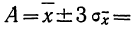
 Значит, истинное значение размера детали находится в границах от 141,5—2,04 до 141,5+2,04.
- Методы математической статистики
- Комбинаторика — правила, формулы и примеры
- Классическое определение вероятности
- Геометрические вероятности
- Законы распределения случайных величин
- Дисперсионный анализ
- Математическая обработка динамических рядов
- Корреляция — определение и вычисление
Теория ошибок измерений изучает свойства ошибок и законы их распределения, методы обработки измерений с учетом их ошибок, а также способы вычисления числовых характеристик точности измерений. При многократных измерениях одной и той же величины результаты измерений получаются неодинаковыми. Этот очевидный факт говорит о том, что измерения сопровождаются разными по величине и по знаку ошибками. Задача теории ошибок – нахождение наиболее надежного значения измеренной величины, оценка точности результатов измерений и их функций и установление допусков, ограничивающих использование результатов обработки измерений.
По своей природе ошибки бывают грубые, систематические и случайные.

Грубые ошибки являются результатом промахов и просчетов. Их можно избежать при внимательном и аккуратном отношении к работе и организации надежного полевого контроля измерений. В теории ошибок грубые ошибки не изучаются.
Систематические ошибки имеют определенный источник, направление и величину. Если источник систематической ошибки обнаружен и изучен, то можно получить формулу влияния этой ошибки на результат измерения и затем ввести в него поправку; это исключит влияние систематической ошибки. Пока источник какой-либо систематической ошибки не найден, приходится считать ее случайной ошибкой, ухудшающей качество измерений.
Случайные ошибки измерений обусловлены точностью способа измерений (строгостью теории), точностью измерительного прибора, квалификацией исполнителя и влиянием внешних условий. Закономерности случайных ошибок проявляются в массе, то-есть, при большом количестве измерений; такие закономерности называют статистическими. Освободить результат единичного измерения от случайных ошибок невозможно; невозможно также предсказать случайную ошибку единичного измерения. Теория ошибок занимается в основном изучением случайных ошибок.
Случайная истинная ошибка измерения Δ – это разность между измеренным значением величины l и ее истинным значением X:
 (1.25)
Свойства случайных ошибок. Случайные ошибки подчиняются некоторым закономерностям:
1. при данных условиях измерений абсолютные значения случайных ошибок не превосходят некоторого предела; если какая-либо ошибка выходит за этот предел, она считается грубой,
2. положительные и отрицательные случайные ошибки равновозможны,
3. среднее арифметическое случайных ошибок стремится к нулю при неограниченном возрастании числа измерений. Третье свойство случайных ошибок записывается так:
 (1.26)
4. малые по абсолютной величине случайные ошибки встречаются чаще, чем большие.
Кроме того, во всей массе случайных ошибок не должно быть явных закономерностей ни по знаку, ни по величине. Если закономерность обнаруживается, значит здесь сказывается влияние какой-то систематической ошибки.
Средняя квадратическая ошибка одного измерения. Для оценки точности измерений можно применять разные критерии; в геодезии таким критерием является средняя квадратическая ошибка. Это понятие было введено Гауссом; он же разработал основные положения теории ошибок. Средняя квадратическая ошибка одного измерения обозначается буквой m и вычисляется по формуле Гаусса:
 (1.27)
где:  ;
;
n – количество измерений одной величины.
Средняя квадратическая ошибка очень чувствительна к большим по абсолютной величине ошибкам, так как каждая ошибка возводится в квадрат. В то же время она является устойчивым критерием для оценки точности даже при небольшом количество измерений; начиная с некоторого n дальнейшее увеличение числа измерений почти не изменяет значения m; доказано, что уже при n = 8 значение m получается достаточно надежным.
Предельная ошибка ряда измерений обозначается Δпред; она обычно принимается равной 3*m при теоретических исследованиях и 2*m или 2.5*m при практических измерениях. Считается, что из тысячи измерений только три ошибки могут достигать или немного превосходить значение Δпред = 3*m.

Отношение mx/X называется средней квадратической относительной ошибкой; для некоторых видов измерений относительная ошибка более наглядна, чем m. Относительная ошибка выражается дробью с числителем, равным 1, например, mx/X = 1/10 000.
Средняя квадратическая ошибка функции измеренных величин. Выведем формулу средней квадратической ошибки функции нескольких аргументов произвольного вида:
F = f( X, Y, Z … ), (1.28)
здесь: X, Y, Z … – истинные значения аргументов,
F – истинное значение функции.
В результате измерений получены измеренные значения аргументов lX, lY, lZ, при этом:
 (1.29)
где ΔX, ΔY, ΔZ – случайные истинные ошибки измерения аргументов.
Функцию F можно выразить через измеренные значения аргуметов и их истинные ошибки:

Разложим функцию F в ряд Тейлора, ограничившись первой степенью малых приращений ΔX, ΔY, ΔZ:
 (1.30)
Разность является случайной истинной ошибкой функции с противоположным знаком, поэтому:
 (1.31)
Если выполнить n измерений аргументов X, Y, Z, то можно записать n уравнений вида (1.31). Возведем все эти уравнения в квадрат и сложим их; суммарное уравнение разделим на n и получим


В силу третьего свойства случайных ошибок члены, содержащие произведения случайных ошибок, будут незначительными по величине, и их можно не учитывать; таким образом,
 (1.32)
Как частные случаи формулы (1.32) можно написать выражения для средней квадратической ошибки некоторых функций:

Если функция имеет вид произведения нескольких аргументов,
F = x * y * z,
то для нее можно записать выражение относительной ошибки функции:
 (1.33)
которое в некоторых случаях оказывается более удобным, чем формула (1.32).
Принцип равных влияний. В геодезии часто приходится определять средние квадратические ошибки аргументов по заданной средней квадратической ошибке функции. Если аргумент всего один, то решение задачи не представляет трудности. Если число аргументов t больше одного, то возникает задача нахождения t неизвестных из одного уравнения, которую можно решить, применяя принцип равных влияний. Согласно этому принципу все слагаемые правой части формулы (1.32) или (1.33) считаются равными между собой.
Арифметическая середина. Пусть имеется n измерений одной величины X, то-есть,
 (1.34)
Сложим эти равенства, суммарное уравнение разделим на n и получим:
 (1.35)
Величина  (1.36)
называется средним арифметическим или простой арифметической серединой. Запишем (1.35) в виде

по третьему свойству ошибок (1.26) можно написать:

что означает, что при неограниченном возрастании количества измерений простая арифметическая середина стремится к истинному значению измеряемой величины. При ограниченном количестве измерений арифметическая середина является наиболее надежным и достоверным значением измеряемой величины.
Запишем формулу (1.36) в виде

и подсчитаем среднюю квадратическую ошибку арифметической середины, которая обозначается буквой M. Согласно формуле (1.32) напишем:

или

Но ml1 = ml2 = … = mln= m по условию задачи, так как величина X измеряется при одних и тех же условиях. Тогда в квадратных скобках будет n * m2, одно n сократится и в итоге получим:
M2 = m2/n
или
 (1.37)
то-есть, средняя квадратическая ошибка арифметической середины в корень из n раз меньше ошибки одного измерения.
Вычисление средней квадратической ошибки по уклонениям от арифметической середины. Формулу Гаусса (1.27) применяют лишь в теоретических выкладках и при исследованиях приборов и методов измерений, когда известно истинное значение измеряемой величины. На практике оно, как правило, неизвестно, и оценку точности выполняют по уклонениям от арифметической середины.
Пусть имеется ряд равноточных измерений величины X:
l1, l2 , …, ln .
Вычислим арифметическую середину X0 = [1]/n и образуем разности:
 (1.38)
Сложим все разности и получим [l] – n * X0 = [V]. По определению арифметической середины n * X0 = [l], поэтому:
[V] = 0. (1.39)
Величины V называют вероятнейшими ошибками измерений; именно по их значениям и вычисляют на практике среднюю квадратическую ошибку одного измерения, используя для этого формулу Бесселя:
 (1.40)
Приведем вывод этой формулы. Образуем разности случайных истинных ошибок измерений Δ и вероятнейших ошибок V:
 (1.41)
Разность (X0 – X) равна истинной ошибке арифметической середины; обозначим ее Δ0 и перепишем уравнения (1.41):
 (1.42)
Возведем все уравнения (1.42) в квадрат, сложим их и получим:
 .
.
Второе слагаемое в правой части этого выражения равно нулю по свойству (1.39), следовательно,
 .
.
Разделим это уравнение на n и учтя, что [Δ2]/n =m2, получим:
 (1.43)
Заменим истинную ошибку арифметической середины Δ0 ее средней квадратической ошибкой  ; такая замена практически не изменит правой части формулы (1.43). Итак,
 ,
,
откуда  ;
;
после перенесения (n-1) в правую часть и извлечения квадратного корня получается формула Бесселя (1.40).
Для вычисления средней квадратической ошибки арифметической середины на основании (1.37) получается формула:
 (1.44)
Веса измерений. Измерения бывают равноточные и неравноточные. Например, один и тот же угол можно измерить точным или техническим теодолитом, и результаты таких измерений будут неравноточными. Или один и тот же угол можно измерить разным количеством приемов; результаты тоже будут неравноточными. Понятно, что средние квадратические ошибки неравноточных измерений будут неодинаковы. Из опыта известно, что измерение, выполненное с большей точностью (с меньшей ошибкой), заслуживает большего доверия.
Вес измерения – это условное число, характеризующее надежность измерения, степень его доверия; вес обозначается буквой p. Значение веса измерения получают по формуле:
p = C/m2 (1.45)
где C – в общем случае произвольное положительное число.
При неравноточных измерениях одной величины наиболее надежное ее значение получают по формуле средневесовой арифметической середины:
 (1.46)
или X0 = [l*p] / [p] .
Ошибку измерения, вес которого равен 1, называют средней квадратической ошибкой единицы веса; она обозначается буквой m. Из формулы (1.45) получаем

откуда  (1.47)
то-есть, за число C принимают квадрат ошибки единицы веса.
Подсчитаем вес P средневесовой арифметической середины. По определению веса имеем:
 (1.48)
Согласно (1.46) и (1.32) напишем:

Подставим сюда вместо mli2 их выражения через вес m2 = C/p , тогда:

Подставим это выражение в формулу (1.48) и получим,
P = [p], (1.49)
то-есть, вес средневесовой арифметической середины равен сумме весов отдельных измерений.
В случае равноточных измерений, когда веса всех измерений одинаковы и равны единице, формула (1.49) принимает вид:
P = n. (1.50)
При обработке больших групп измерений (при уравнивании геодезических построений по МНК) вычисляются значение ошибки единицы веса, веса измерений и других элементов после уравнивания, а ошибка любого уравненного элемента подсчитывается по формуле:
 (1.51)
где pi – вес i-того элемента.