Как действует система при возникновении ошибки е

Я пришел на лекцию по моему питону для начинающих, где определенная тема не была объяснена достаточно хорошо. Так что же это e делает?

def x(a, b):
    try:
        return a / b

    except ZeroDivisionError, e:
        return 0

4 ответа

Лучший ответ

Пойманное исключение присваивается имени e. Вы можете выбрать любой действительный идентификатор Python:

except ZeroDivisionError, caught_exception:

Это позволяет вам использовать пойманное исключение; возможно, чтобы напечатать сообщение об ошибке, или использовать атрибуты исключения для других целей. См. главу по обработке исключений учебника по Python.

Синтаксис except <Exception>, <name>: устарел в пользу:

except ZeroDivisionError as e:

Который гораздо более читабелен и позволяет избежать путаницы с синтаксисом для отлова нескольких типов исключений:

except (ZeroDivisionError, ValueError):

Поскольку функция, которую вы опубликовали в противном случае, не использует e, ее можно полностью удалить:

def x(a, b):
    try:
        return a / b
    except ZeroDivisionError:
        return 0

Martijn Pieters
11 Ноя 2013 в 21:04

Сохраняет сообщение, сгенерированное захваченной ошибкой, в имя e. Ниже приведена демонстрация:

>>> 1/0
Traceback (most recent call last):
  File "<stdin>", line 1, in <module>
ZeroDivisionError: integer division or modulo by zero
>>>
>>> try:
...     1/0
... except ZeroDivisionError, e:
...     print e
...
integer division or modulo by zero
>>>

Вы должны отметить две вещи, однако. Во-первых, вам не нужно использовать имя e. Вы можете выбрать любое имя переменной. Во-вторых, приведенный вами синтаксис устарел в пользу:

except Exception as e:

Кроме того, я хотел бы добавить, что ваша конкретная функция может быть переписана так:

def x(a, b):
    return a/b if b else 0

Наличие блока try / Кроме того, что нет необходимости, а наличие e действительно не нужно, так как функция никогда не использует его.

Возможно, будет проще использовать новый синтаксис:

except ValueError as e:
    print e

Который читается более четко — вы собираетесь дать исключению имя, в данном случае просто e. См. это руководство по обработке ошибок.

ratatoskr
11 Ноя 2013 в 20:56

Поскольку ZeroDivisionError не очень хороший пример для объяснения цели «е» (может быть причиной того, почему вам это не ясно), я собираюсь объяснить с другой ошибкой

Исключение: в общем, когда программа Python сталкивается с ситуацией, которую она не может продолжить (глючный код), она вызывает исключение. Исключением является объект Python, который представляет ошибку.

В вашем интерпретаторе Python, если вы делаете что-то с неопределенной переменной (или экземпляром), вы получаете ошибку, подобную этой

>>> a = 1
>>> print a
1
>>> print b
Traceback (most recent call last):
  File "<stdin>", line 1, in <module>
NameError: name 'b' is not defined
>>>

NameError — это имя возникшего исключения

имя ‘b’ не определено — дополнительная информация для возникшего исключения

Давайте повторить то же самое с try и кроме блока

>>> 
>>> 
>>> try:
...     print a
...     print b
... except NameError:
...     print "I got NameError"
... 
1
I got NameError
>>>

Вывод не является явным о переменной / экземпляре, вызывающем это исключение. Вы можете чувствовать, что вы можете справиться с этим, если у вас есть доступ к дополнительной информации, предоставленной переводчиком

Вот где необязательный аргумент ( кроме ) «e» или все, что вы хотите вызвать, становится удобным

>>> try:
...     print a
...     print b
... except NameError, e:
...     print "I got NameError"
...     print "Addition Information is:", e
...     
... 
1
I got NameError
Addition Information is: name 'b' is not defined
>>>

Как указано другими, рекомендуем использовать следующую конвенцию

 except NameError as e

user2390183
12 Ноя 2013 в 00:23

Источник

Содержание

Устройство и принцип работы газовых котлов Electrolux
Причины и виды неисправностей в котле
Вероятные ошибки и причины возникновения
Основные коды ошибок газовых котлов «Электролюкс» (Electrolux)
Нарушения в работе с кодом Е4
Ошибка Е3 котла Электролюкс Оставить
Нарушения в работе с кодом Е4

Котел Электролюкс: ошибка Е2

Ассортимент газовых котлов компании Электролюкс впечатляет. Каждая модель относится к одноконтурному или двухконтурному типу газового котла. При этом для каждого предусмотрена установка открытой или закрытой камеры сгорания.

Преимущества:

наличие погодозависимой системы управления ЕТС позволяет устанавливать комфортную температуру нагрева, основываясь на погодных условиях. Также защищает технику от замерзания, перегрева, влияния экстремальных погодных условий;
возможность установки времени работы системы с необходимыми временными интервалами, что помогает экономить воду и электроэнергию;
надежная система защиты котла – выключение в случае плохого дымоотвода, повышенной загазованности и пр.
высокая производительность при скачках в подаче воды, электроэнергии – КПД 94%.

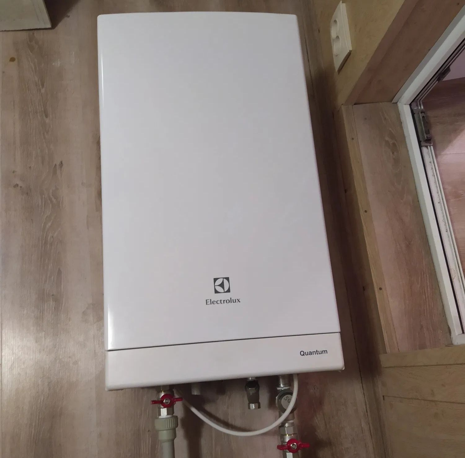
Оптимальный вариант для домашней отопительной системы – двухконтурный газовый котел. Универсальность техники заключается в одновременном отоплении всей площади дома и бесперебойной подаче горячей воды в систему водоснабжения. Настенный газовый котел «Электролюкс» удобен в последующей установке, так как снизу корпуса расположены все необходимые патрубки ввода и вывода отопительной воды.

Составляющие сектора гидравлики – реле давления, трехходовый клапан, циркуляционный насос, клапан сброса, вторичный пластинчатый обменник, расширительный бак. «Внутренности» газового тракта – рабочий клапан, инжекционная нержавеющая горелка, электроды зажигания и регуляции подачи пламени, стальная топка с гидроизоляцией, первичный теплообменник. Датчик теплообменника сохраняет систему от резких перегревов и закипания.

Дополнительно оборудование оснащено вентилятором для удаления «отходов» горения и нормализации давления.

Причины и виды неисправностей в котле

Важнейшим элементом в функционировании котла является электронная плата управления, которая контролирует работу и вовремя сообщает о возникших неисправностях. Каждая ошибка имеет свой специальный код, выводящийся на ЖК-дисплей устройства, либо сообщающиеся индикацией на панели прибора.

Для отопительных приборов ошибки делятся на 2 группы:

аварийные, при которых функционирование полностью останавливается до исправления;
информационные, когда устройство ждёт выполнения необходимых действий и переходит в ожидание.

Вероятные ошибки и причины возникновения

В этой статье собраны все вероятные неисправности и варианты их устранения, а так же коды ошибок для котлов Электролюкс (Electrolux). Вся информация читается в следующем порядке: код — наименование — возможная неисправность.

Коды ошибок, возможные при работе модели Electrolux Basic
Код ошибки Е1 — Ошибка подачи газа
Код ошибки Е2 — Ошибка подачи воды в систему
Код ошибки Е3 — Ошибка вентилятора, дымохода или электроники
Код ошибки Е4 — Ошибка давления
Код ошибки Е6 — Ошибка датчика ГВС или электроники
Код ошибки Е7 — Ошибка датчика температуры воды или электроники
Возможные коды ошибок и поломки моделей Electrolux hi-tech
Код ошибки Е1 — Нет пламени
Код ошибки Е2 — Перегрев теплоносителя
Код ошибки Е3 — Проблемы с удалением продуктов горения из котла
Код ошибки Е4 — Давление в системе отопления находится ниже предельно допустимого значения
Код ошибки Е6 — Проблемы с работой датчика температуры ГВС
Код ошибки Е7 — Проблема с работой датчика температуры теплоносителя
Код ошибки Е9 — Замерзание системы отопления

Если вы на 100% не уверены в чем именно проблема и в том, что вы сможете ее решить — немедленно обратитесь в сервисный центр для диагностики и устранения неисправности.

Основные коды ошибок газовых котлов «Электролюкс» (Electrolux)

Цифровой ЖК-дисплей расположен спереди корпуса газового котла Электролюкс. Отображает показатель действующей температуры на теплоносителе, параметры работы системы и определенный код ошибки, в случае возникновения неисправности.

Практически все неполадки можно устранить самостоятельно, но в случае непрерывного возникновения новых неисправностей и поломок, следует обратиться за ремонтом к специалисту. Частые неисправности:

отсутствие подачи пламени или её нестабильность (е1);
перегрев теплоносителя (е2);
плохой дымоотвод и поломка в работе составляющих дымоудаления (ошибка е 3).

Рассмотрим причины появления показателей наличия неисправностей и возможные схемы ремонта.

е1:

Причины появления на панели ошибки е1 кроятся в сниженном давлении в газовой магистрали или неисправности электрода розжига, из-за чего не поступает подача пламени. Что можно сделать:

Проверить вентиль, провернуть его до упора.
Перезапустить оборудование нажатием кнопки «reset». Если котел не запустился, то обратитесь за помощью в сервисный центр.
Проведите диагностику электрода: очистите его от грязи, отрегулируйте его местоположение.
Проверьте провода на исправность: осмотрите на наличие дефектов, повреждений и пр.
Осмотрите клапан газа, в случае его неисправности замените деталь новой.
Продиагностируйте плату управления. В случае повреждений замените её.
Если, после диагностики вышеупомянутых составляющих, газовый котел по-прежнему не работает, необходимо обратиться к специалисту. Возможная причина в данном случае – воздушные пробки в газовой магистрали.

е2:

Выявленная на дисплее аппарата Электролюкс ошибка e2 предупреждает пользователя о нагреве теплоносителя, который происходит в случае большой завоздушенности в трубах, поломки циркуляционного насоса, низкого давления в магистрали. Также проблемой данной ошибки может быть закрытый или открытый не полностью газовый вентиль.

Вентиль подачи газа

Методы устранения:

открыть вентиль до упора для подачи газа;
устранить завоздушенность путем открытия кранов отвода воздуха и дыма;
перезапустите оборудование при возникновении соответствующего параметра на дисплее. Если котел не
включился, то прозвоните датчик мультиметром;
проверьте систему на наличие течи, налив воду в бак;
продиагностируйте работу насоса, прозвоните контакты. Если показатель напряжения отличается от нормы, то установите стабилизатор.

В большинстве случаев требуется замена составляющих оборудования. Приобрести запчасти к газовым котлам можно в сервисном центре производителя, либо в специализированном магазине автозапчастей. Также доступно оформление заказа через магазин, где был куплен аппарат.

е3:

Значение параметра ошибки e3 – неисправность дымоотвода. Оборудование автоматически блокируется и отключается, так как при засоре в дымоотводе или резких перепадах температур срабатывает датчик системы безопасности.

Дымоход

Причины и способы решения данной проблемы:

Проведите проверку и чистку дымоотвода. Если он коаксикального типа, то требуется регулярное удаление накопившегося льда или снега зимой.
Продиагностируйте контакты питания датчика на возможные дефекты. В случае окисления проводов необходимо их почистить и восстановить подключение.
Проверить термодатчик на возможность короткого замыкания. При неисправности – заменить его.
Необходимо продиагностировать контакты платы газового котла Электролюкс. Если деталь не работает, то заменить новой.
Наладьте приточную тягу воздуха в помещении. Помните, что работа кондиционера или вентилятора мешает правильной работе всей отопительной системы. Лучше откройте форточку или дверь.
Неправильная сборка дымоотводной системы приводит к наличию подобной неисправности. В некоторых случаях может потребоваться полный демонтаж конструкции и обновленная сборка, следуя определенным параметрам.

е4:

Значение ошибки е4 – падение давления в магистрали ниже нормы в 1 Бар. Причиной может быть поражение теплообменника накипью или поражение радиатора коррозией, после которой появилась протечка воды. Что можно сделать:

выключить аппарат и открыть топливный вентиль для падения параметра давления на манометре. После процедуры включите оборудование;
если ошибка остается на дисплее, необходимо очистить радиатор от накипи с помощью раствора лимонной кислоты;
паяльником можно самостоятельно устранить отверстия, дающие течь в радиаторе.

е5:

Показатель повышенного давления в магистрали выше 2,5 Бар.

Давление в магистрали

Возможно, ошибка появилась из-за неправильной работы датчика давления. В другом случае причина в дефекте защитного клапана. Как ремонтировать:

перезапустить котел с помощью кнопки «reset», если показатели на дисплее не изменяются, то перейти к следующим пунктам;
промыть фильтр предохранительного клапана;
проверить расширительный бак на наличие поломки;
продиагностируйте контакты датчика на перенапряжение или обрыв, если неисправны – замените деталь.

е6:

Поломка сенсора подачи горячего водоснабжения. Необходимо перезапустить устройство для выявления точно проблемы:

если котел не начинает свою работу, то необходимо заменить датчик;
если код ошибки остается неизменным, нужно провести диагностику контактов, соединительных проводов сенсора; проверить плату системы, если неисправна – заменить.

е9:

Причина – в понижении температуры в котле ниже 2 градусов. Для устранения дальнейших показателей данного кода и устранения возможного замерзания необходимо установить дополнительный термометр на улицу, чтобы следить за состоянием температуры. Если котел не будет использоваться в зимний период, слейте воду, как указано в инструкции по эксплуатации оборудования.

Дополнительно проводится настройка газового котла Электролюкс «Басик» при наличии подобной проблемы и после длительного выключения.

Нарушения в работе с кодом Е4

Бытовое газовое оборудование требует от владельцев регулярного осмотра и пристального внимания. Ведь малейшая неполадка может обернуться серьезной бедой. От безвозвратно утраченного оборудования до отравлений разной степени и взрывов с пожарами – все это последствия незначительных, на первый взгляд, поломок.

Изготовители агрегатов для обслуживания частных контуров отопления и ГВС прекрасно понимали, что не все из хозяев техники будут подготовлены к их эксплуатации на профессиональном уровне. Потому и была разработана система предупреждений, высвечивающихся на дисплеях котлов.

Для того чтобы с управлением и настройкой котлов нового поколения мог справится пользователь без специализированного образования и подготовки, агрегаты оснащаются электронными устройствами управления с дисплеями. Во время настройки на электронном экране газового котла отображаются функции и параметры, благодаря чему пользователю значительно легче выбрать необходимый ему режим. У владельца газового котла есть возможность постоянно отслеживать рабочие характеристики газового оборудования, чтобы своевременно принять меры в случае назревания или появления поломки. В случае нарушения работоспособности газового прибора пользователь сразу получит сигнал в виде набора цифр и букв, по сути являющихся автоматической самодиагностикой. Газовые котлы нового поколения. Облегчение процесса настройки параметров. Демонстрация рабочих характеристик. Своевременный сигнал об ошибке

Плохо одно: буквенно-цифровое обозначение поломки котла практически у всех марок свое. В чем-то системы расшифровки перекликаются, но в основном различаются. Коды ошибок оборудования с логотипом Bosch, к примеру, абсолютно неприемлемы для диагностики поломок котлов Viessmann или приборов Ariston.

Как поступить в непростой ситуации, если ваша газовая колонка упорно сигналит, высвечивая ошибку Е4? Проще простого – разобрать все типичные варианты сбоев в работе нагревательной техники, чаще всего приобретаемой нашими соотечественниками.

В качестве примера рассмотрим настенные модели шведского производства с логотипом Elektrolux. Точнее, разберем нарушения в функционале агрегатов с указанным типом ошибки.

Прославленный поставщик качественной и надежной техники разработал единую систему оповещения об ошибках для одноконтурных приборов с закрытой камерой сгорания (Basic S Fi), для двухконтурных моделей с закрытой (Basic Space Fi, Basic X Fi) и открытой (Basic Space i) камерой сгорания.

Аналогичные коды используются в оповещении и расшифровке ошибок агрегатов Электролюкс серий Magnum, Basic Duo, Quantum.

К причинам отображения на электронном табло кода Е4 в перечисленных моделях относятся:

Низкое давление в подключенном к котлу отопительном контуре.
Отсутствие контакта между датчиком давления и внутренней проводкой котла.
Поломка циркуляционного насоса.

Во всех перечисленных случаях команду на блокировку работы котла отдал датчик давления. Тут два варианта: или по контуру слабо циркулирует теплоноситель, или он сам некорректно снял показания. Искать причину начнем с самого распространенного нарушения – проверим давление в обслуживаемом котлом контуре отопления.

Если на электронном дисплее котла значится давление в 0,5 бар, попробуем сначала перезапустить котел. Не исключено, напора, достаточного для нормального движения теплоносителя через теплообменник нет из-за нарушения электрической цепи или поломки насоса.

Ошибка е04 на дисплее котла Электролюкс
На дисплее котлов марки Электролюкс код Е04 появляется, если затрудняется циркуляция нагретой воды или некорректно работают устройства регистрации данных и управления

О том, что внимания, ремонта/замены заслуживает насос или подсоединенная к нему электропроводка, подскажет повышение значения давления после перезапуска как минимум на 0,1 бар. В обоих случаях следует обратиться к газовщикам, с которыми заключен договор на поставку газообразного горючего и техобслуживание агрегата.

Ошибка Е3 котла Электролюкс Оставить

Котел электролюкс ошибка е3 что делать?
Ошибка Е3 котла Electrolux

Недостаток заводских инструкций на импортное оборудование – в минимуме информации в разделе «Диагностика», полезной для пользователя. После указания вероятной причины появления кода неисправности следует общая рекомендация: обращайтесь к сервисному специалисту.

Ошибка е3 котла Электролюкс не самая сложная, и в большинстве случаев устраняется своими силами. Что можно сделать самому, читатель узнает из этой статьи.

На заметку! Поиск причин появления любой ошибки котла нужно начинать со сброса (копка REZET на лицевой панели Электролюкс). При скачках напряжения питающей сети автоматика выдает на дисплей ложный код, хотя на самом деле никакой проблемы с котлом или системой отопления нет. Но если ошибка не исчезает, нужно разбираться с причинами, ее вызвавшими. И не всегда они связаны с поломками отопительной установки.

Кнопка Reset на панели управления котлом Electorlux Biasi

Код е3 котла Электролюкс информирует пользователя о неполадках в системе дымоудаления.

Следовательно, круг поисков сужается – контур отопления при такой ошибке тестировать не нужно.

Тестирование простое – на предмет наличия/отсутствия тяги. Контроль осуществляется по язычку пламени: свечи, зажигалки, спички. Степень засорения, конкретный участок можно определить с помощью зеркальца. Если оголовок дымохода не обустроен должным образом, канал постепенно забивается пылью, листвой, иногда залетевшей мелкой птахой. Самостоятельно прочистить, устранив тем самым ошибку е3 котла, сможет каждый.

Коаксиальный дымоход с защитой от внешней среды

Несколько сложнее для Электролюкс с коаксиальным дымоходом. В зимнее время при нарушении правил монтажа системы дымоудаления наблюдается оледенение канала. Придется отогревать, а чем именно, решается на месте.

В первую очередь оценивается состояние сигнальных линий, цепей питания. Наиболее вероятные причины любой из ошибок котлов: обрывы, замыкания, оплавление изоляции

Электролюкс серии Атмо

В котлах этой модификации продукты горения отводятся естественным путем. И если с каналом дымоудаления проблем нет, нужно смотреть датчик тяги. Его чувствительный элемент – биметаллическая пластина. Вероятная причина ошибки е3 – отсутствие сигнала на электронную плату из-за проблемы с контактами (тип НЗ) или проводами (обрыв, замыкание). Датчик ремонту не подлежит, только замена.

Датчик предназначен для контроля тяги в газовых котлах Electrolux

Электролюкс серии Турбо

Вентилятор. Механическая часть проверяется легким прикосновением к крыльчатке: она должна свободно вращаться. Состояние обмотки несложно оценить подачей напряжения питания напрямую.
Устройство Вентури. Его назначение – контроль потока дымовых газов. Состоит из силиконовой трубки, работающей совместно с датчиком-прессостатом. По ней на его мембрану передается давление, что вызывает срабатывание микровыключателя. В первую очередь нужно внимательно осмотреть пластиковый корпус датчика и полимерную трубку. Температурная деформация – повод заменить. Далее проверяется трубка: она нередко забивается копотью, пылью, и канал блокируется.
Прессостат. В документации обозначается еще и как датчик дыма, реле давления дифференциальное. При включении вентилятора его НР (нормально разомкнутые) контакты замыкаются от воздействия мембраны (она изгибается), и на электронную плату котла поступает сигнал, что проблем с вытяжкой нет. Прессостат не ремонтируется, меняется.

Если принятые меры не дали положительного результата, остаются две причины появления кода е3 Электролюкс: неисправность в плате управления котла и ошибки в расчете параметров дымохода.

В последнем случае могут быть неверно определены диаметр, общая протяженность магистрали, количество поворотов, длина вертикального, «разгонного» участка (для Электролюкс Атмо). Выяснить, где проблема, сможет только профильный специалист.

Периодическое высвечивание ошибки е3 с остановкой котла, наблюдающееся лишь при сильных порывах ветра, изменении направления – явный признак просчетов, допущенных при составлении схемы дымохода и его монтаже.

Нарушения в работе с кодом Е4

Источники

https://WyseDevice.ru/uborka/elektrolyuks-oshibka-e4.html
https://m-strana.ru/articles/kotel-baksi-oshibka-e01/
https://kuban-stan.ru/kak-chinit/kotel-elektrolyuks-oshibka-e2.html
https://KTexnika.ru/uborka/oshibka-e2-elektrolyuks.html
https://sovet-ingenera.com/otoplenie/kotly/oshibka-e4-v-gazovom-kotle.html
https://megavat116.ru/kotel-elektrolyuks-oshibka-e3-chto-delat/

Источник

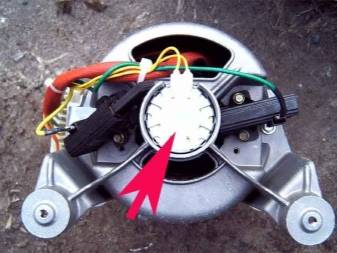
Тестируем двигатель

О чем свидетельствует данное кодовое обозначение? Ошибка E02 сигнализирует о неисправности электродвигателя СМА или управляющей платы. На большинстве Электролюксов установлен коллекторный движок, проверку которого можно произвести своими руками.

Что делать перед тем, как протестировать мотор? Изначально необходимо разобраться со схемой подключения двигателя. Большая часть коллекторных движков имеют довольно простую схему.

В стиральных машинах Электролюкс для переключения обмотки статора используется реле, и применяются контакты командоаппарата. Описанные комплектующие располагаются в управляющем модуле стиральной машины.

Обмотка статора разделена на 2 секции. Данная конструктивная особенность уменьшает влияние помех, периодически возникающих вследствие появления искр на коллекторе.

Барабан любой стиральной машины попеременно вращается в разные стороны. Это движение обуславливается сменой полярности обмотки статора. В некоторых моделях предусмотрен отдельный отвод для обмотки, он активируется при отжиме вещей. В таком случае, электрический ток подключается к любому из крайних выводов и данному отводу. На этапе основного процесса стирки статорная обмотка включается через крайние выводы, это обеспечивает неспешное, плавное вращение барабана.

Чтобы проверить двигатель и отыскать решение проблемы, необходимо произвести соединение обмотки ротора и статора поочередно, и включить их в электросеть. Наглядно данная схема подключения представляется следующим образом:

Данный способ диагностики характеризуется некоторыми недостатками. Во-первых, выбирая такой метод проверки, у вас не будет возможности убедиться в исправности мотора на 100%. Штатное вращение вала не сможет гарантировать, что на различных этапах стирки машинка Электролюкс не выдаст какой-либо сбой.

Помимо этого, подключение элементов по такой схеме не предусматривает защиты. Поэтому, если при проверке движок «коротнет», он, скорее всего, просто выйдет из строя. Чтобы предохранить электродвигатель от возможных повреждений, в схему лучше включить дополнительное звено. В качестве добавочного элемента можно использовать ТЭН стиральной машинки или просто светильник высокой мощности (более 500 Вт). Схема будет выглядеть следующим образом:

Балласт, включенный в соединение, защитит тестируемый движок. При возникновении замыкания, ток пойдет на ТЭН, который начнет нагреваться.

Существует и другой способ диагностики двигателя в стиральной машине Электролюкс. Статорные и роторные обмотки соединяются аналогично второй схеме, только запитываются они специальным лабораторным трансформатором, мощностью свыше 500Вт. Преимуществом метода является возможность постоянно контролировать число оборотов и своевременно принимать меры при каком-либо сбое. Для большей безопасности допускается использование предохранителя с пропускной способностью 5-10 Ампер.

Вместо автотрансформатора разрешено применить для диагностики электронный регулятор, который обычно используется, чтобы контролировать нагрузки данной мощности. В таком случае лучше обратиться за помощью к специалистам, но если у вас имеются определенные познания в электронике, диагностику и ремонт можно провести самостоятельно.

Еще один вариант проверки мотора – наблюдение, насколько сильным и ярким будет искрение между щетками и коллекторным движком. При значительном искрении вероятно, двигатель стиралки неисправен.

Именно вышеназванными способами допускается проверить электродвигатель машинки-автомата, отображающей ошибку E02

Если после проведения диагностики движка найти решение проблемы не получилось, следует переходить к проверке другого важного элемента системы

Сгорел симистор контролирующий УБЛ

Вторая возможная причина при появлении ошибки E41 – сгоревший симистор или неисправная плата управления. То есть УБЛ работает нормально, но система не получает сигнал о произошедшей блокировке. Чтобы починить испорченный модуль, схему придется достать и осмотреть. Для этого необходимо:

вынуть диспансер для моющих средств, покачав лоток и с усилием потянув его на себя;
найти в отверстии рядом с отсеком для кюветки 2 болта и открутить их;
достать еще 4 винта, расположенных на торце панели под верхней крышкой автомата;
взять панель руками и аккуратно сдвинуть вверх;
поддеть плоской отверткой фиксаторы-защелки;
разобрать корпус панели и достать управляющую плату.

Как только плата оказалась в руках, стоит внимательно осмотреть ее поверхность на дефекты, следы горения или механические повреждения. Если видимых причин для беспокойства нет, придется вновь прибегнуть к помощи мультиметра и проверить каждый симистор на пробой. Следующая инструкция поможет понять, что делать для проверки модуля.

Переводим тестер в режим звуковой прозвонки.
Касаемся щупами контактов А1 и А2 и смотрим на экран. При высвечивании «1» или «OL» – симистор исправен, а когда число близко к нулю – необходимо исправить ситуацию заменой детали.
Когда ТЗ между выводами нет, проверяем управляющий электрод. Направляем концы прибора к силовым выводам и основному электроду. При значениях в 80-200 беспокоиться не о чем.
Замыкаем главный электрод, а после пары секунд убираем ток, наблюдая за состоянием симистора. Если переключатель не закрылся, то требуется полноценный ремонт с заменой.

Но лучше с платой не экспериментировать и доверить решение проблемы с ошибкой E41 мастерам сервисного центра. Помните, что модуль – вещь хрупкая и дорогая, поэтому без опыта и практики легко усугубить поломку.

Что нужно делать при ошибках

Если на дисплее появился код ошибки, нужно его расшифровать и немедленно обесточить машину.

Важно понять значение ошибки и причины ее появления на дисплее.

Затем нужно действовать, исходя из вида неисправности:

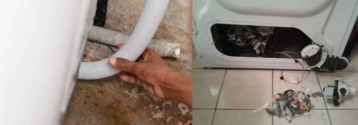
Е20: отсоединяем сливной шланг, сливаем воду. Если слив затруднен, его нужно прочистить. После прочистки ошибка может исчезнуть. Также может быть загрязнен фильтр. Его следует проверить. Забиться может и помпа. Ее чистку лучше доверить профессионалу, если нет уверенности в своих силах;
Е10: Для начала нужно проверить напор воды из крана. Чаще всего причина заключается в самом простом. Затем нужно осмотреть заливной шланг на целостность, на отсутствие зажима. Если проблема не в этом, то лучше обратиться к профессионалу. Самостоятельно качественно прочистить фильтр или отремонтировать модуль управления проблематично;
Е40: Если диагностика показала, что неисправен замок дверцы, то его ремонт можно осуществить заменой на новый. Для этого следует снять хомут, выкрутить болты, снять замок, отсоединить все проводки, установить новый. Если проблема заключается в неисправности электрической цепи, то нужно проверить все проводки, прозвонив их мультиметром;
Е13: Чаще всего причиной данной поломки является износ одного из шлангов. Нужно тщательно проверить оборудование на предмет протечки воды;
Машинка не забирает порошок. Данную неисправность техника обнаружить не в состоянии. Найти неиспользованный гель или порошок может только сам пользователь. Чаще всего причиной этой неисправности является засор дозатора. В этом случае машину нужно отсоединить от электропитания, полностью достать лоток, промыть его под проточной водой.

Причины

Каждый из кодов ошибки имеет причину (и чаще не одну) возникновения. Так, код ошибки E11 обычно возникает при поломке одного из клапанов залива воды или схемы его управления на электронном контроллере. Эта наиболее распространенная, но не единственная причина. Среди прочих – недостаточное сопротивление обмотки клапана (норма – 3,75 ОМ), недостаточное давление воды в водопроводных трубах, засорение тракта залива воды.

При возникновении проблем со сливом воды (код ошибки Е21) стоит проверить исправность сливного насоса, проходимость фильтров, патрубка и сливного шланга. Именно неисправности и засоренность этих элементов и узлов машинки чаще всего становятся причиной подобного рода поломки. Также есть смысл проверить напряжение обмотки сливного насоса (норма – 170 Ом). Наконец, причиной подобного рода ошибки может стать и неисправность электронного контроллера.

С превышением времени слива может быть связана и ошибка EF1, а высвечивание кода EF2 сигнализирует о повышении пенообразования, первопричиной которого также является засор сливной магистрали. Истоки проблемы в таком случае ищут в сливном шланге или канализации, есть смысл проверить на наличие засора фильтр над сливной помпой.

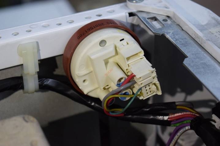
Причины поломки прессостата вызывают в основном засорение трубки, сбои в работе электросети, сбои в настройках программ. Прессостат отвечает за общую работоспособность стиральной машинки, иначе его называют датчиком воды и датчиком напряжения. Вот почему выход из строя этого элемента приводит к появлению совершенно разных «симптомов» – преждевременный запуск стирки, невозможность активации функции отжима белья.

Причины возникновения ошибок Е40-Е43 связаны с неплотно закрытой дверцей люка. Это может быть попадание в замок мусора, инородных предметов. То есть поиск причины неисправности начинается именно с этой зоны. Если с замком все в порядке, то причиной появления данных кодов ошибки может стать перекос дверцы. То есть винтики в болтиках разболтались, дверца «съехала», поэтому закрыть ее правильно невозможно. Понятно, что в этом случае следует отверткой потуже затянуть болтики и вернуть дверце нужное положение.

Иногда причина неплотно закрытой дверцы может скрываться в перепадах напряжения. Проверить это можно простым способом – отключить стиральную машинку из электросети на 10-15 секунд, а затем включить вновь. Как вариант – попробовать вручную прижать дверцу к люку руками и подождать, не раздастся ли характерный щелчок и не появится ли на дисплее значок блокировки.

Наконец, причиной неплотного закрывания дверцы может стать износ деталей машинки. В среднем все они рассчитаны на 5-летний срок службы. Неполадки работы электродвигателя можно выявить по возникновению на дисплее ошибки Е50. Причем причиной ее возникновения может быть неисправность реле, подшипников, отсутствие сигнала от тахогенератора.

Одним из слабых мест стиральных машин является ТЭН. Одна из частых причин выхода из строя нагревательного элемента – образование накипи на его поверхности. Накипь не пропускает тепло, то есть ТЭН начинает перегреваться, а нагрев воды при стирке оказывается недостаточным.

Иногда ТЭН, напротив, слишком быстро и сильно нагревает воду. В данном случае «виноват» температурный датчик, который следует заменить. Могут выйти из строя и реле, управляющие функционированием нагревательного элемента.

Устранение

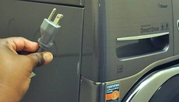
Итак, одной из распространенных проблем является отсутствие сигналов на дисплее при включении машинки в сеть. Проще говоря, она никак не реагирует на подобные действия. В первую очередь следует проверить, есть ли электричество в сети – включить другую технику в розетку.

Если все в порядке, проверьте сетевой шнур и вилку. При обнаружении повреждений не изолируйте, а замените. Причиной может стать и окисление контактов панели управления или перегорание сетевого фильтра или его элементов Устранение данного типа неполадок начинается со снятия верхней крышки (достаточно открутить болты). Фильтр вы увидите у стенки. При его перегорании будут заметны вздутости. В этом случае фильтр подлежит замене. Для проверки клавиш нужно сначала извлечь лоток, после чего будут видны кнопки (за модулем).

При проблемах с забором и сливом воды первое, что нужно делать – перекрыть запорный вентиль и открутить шланг от корпуса. За ним обнаружится фильтр, его извлекают и промывают под водой, это же следует сделать со шлангом. Есть смысл сразу демонтировать заднюю крышку и проверить мультиметром расположенный за ним впускной клапан (норма – 2-4 Ом).

Если вода осталась в баке, следует также прочистить слив. Обнаружить его можно за дверцей, расположенной в нижней части машинки (с фронтальной стороны). Открыв эту дверцу, вы увидите фильтр, который нужно открутить

Внимание, в этот момент из отверстия польется вода, поэтому следует сразу подготовить ветошь и ведра. Открутив фильтр, его промывают, а также пространство, которое он закрывает

Если барабан стал плохо отжимать белье, а машинка сильно вибрировать, следует проверить натяжение приводного ремня. Для этого нужно открутить заднюю панель устройства. Если ремень слетел, вы сразу это увидите, достаточно вернуть его на место (на шкив двигателя). При износе ремня он подлежит замене. В машинах с классическим двигателем может потребоваться замена щеток. Проверить нужно их графитовые стержни (извлечь из корпуса, отключив контакты).

О том, как прочитать код ошибки в стиральных машинах, смотрите в следующем видео.

Все элементы исправны, но сигнал ошибки не исчезает

Как исправить проблему, мы разобрались. Но порой возникает такая ситуация, при которой известная нам ошибка способна нарушить работу машины для стирки белья без причин. Выражаясь точнее, проблема все же существует, но с поступлением или спуском жидкости она не связана, и агрегаты, отвечающие за это, функционируют нормально. Получается, что машина стирает, но на экране высвечивается тревожный сигнал.

Причиной его появления может оказаться электроника. Если говорить конкретно – управленческий блок. Выйти из строя он может по нескольким причинам – от перепадов напряжения, от частых остановок машины во время рабочего процесса, от наличия заводского брака и т. п.

Разобраться в этом случае с такой ситуацией придется опытному специалисту, так как самому демонтировать и тестировать модуль блока управления не рекомендуется, если для этого нет соответствующих навыков.

Информация об уровне воды

Модели стиральной машинки фирмы «Самсунг» оснащены специальным прессостатом, который контролирует заполнение барабана водой. Когда прессостат не получает нужный для начала работы сигнал, дисплей выдает ошибку.

E7

О зашифрованной ошибке оповещение поступает от датчика (прессостата) уровня воды. К появлению данного цифробуквенного значения на дисплее приводит поломка самого датчика либо нарушение целостности трубки, которая соединяет датчик с барабаном.

1C

Если высветился код 1C, то возникла одна из следующих проблем:

поломка датчика, контролирующего уровень поступающей воды;
дефекты соединительных контактов;
поврежден, загрязнен или изогнут участок трубки, принадлежащий датчику;
поломка системы управления.

1E

Шифр ошибки часто возникает в результате элементарного сбоя в функционировании системы управления. Тогда достаточно будет выключить бытовой прибор из сети и включить через 6 минут снова. Кроме этого, причиной ошибки становится:

отхождение контактов управляющей панели или прессостата;
неполадки, связанные с трубкой, соединяющей датчик с баком отбора давления.

Значение кода ошибки E40

В каждой модели стиральной машины Electrolux такое сочетание буквы и цифр, как E40, сообщает о проблемах с блокиратором загрузочной дверцы. Код имеет общее понятие. Чтобы конкретизировать виновника неисправности, следует войти в режим. Отлично справляется с такой задачей мастер, но алгоритм общих действий выглядит следующим образом:

одновременно нажимаются две кнопки, расположенные справа на управленческой панели;
продолжая их удерживать, необходимо нажать большую кнопку оранжевого цвета, находящуюся сбоку. Давить продолжаем до тех пор, пока не засветятся индикаторные лампочки.

Данный метод рекомендован к применению на машинах, не оснащенных селекторными программами. В случае, если таковой имеется, следует одновременно активировать и не отпускать некоторое время пару крайних кнопок, расположенных справа.

В конечном итоге на экране высветится уточненный код неисправности E40:

E41 – загрузочный люк закрыт не достаточно плотно;
E42 – отказал замок;
E43 – в управленческом модуле сломалась деталь, отвечающая за блокировку;
E44 – неисправность датчика двери;
E45 – возникли проблемы в проводке, соединяющей УБЛ и управленческий блок.

Коды ошибок Электролюкс и их устранение

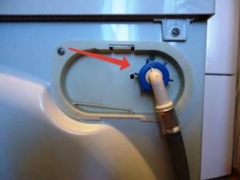
Что делать если стиралка не сливает? Как было сказано выше, причина может быть именно в помпе, которая отвечает за слив воды.

Есть такие ошибки, которые можно легко устранить, не применяя никаких инструментов

Для этого потребуется подготовить:

Крестовую отвертку;
Мультиметр.

Для непосредственного очищения помпы проводится откручивание крышки и проверяется крыльчатка. Вполне возможно, что на ней присутствует осадок в виде волос, шерстяных ниток и тому подобных загрязнений. Мусор счищается максимально аккуратно, что возможно сделает помпу работоспособной. Для диагностики нужно приложить щуп к поверхности помпы и посмотреть на экран мультиметра. Если деталь работает, то устройство выдаст результат в 200 Ом, а при его отсутствии потребуется замена насоса на аналогичную модель подходящую именно к данному устройству для стирки белья.

Как только помпа заменена, проводится запуск оборудования обязательно в режиме тестирования, чтобы отследить грамотность работы изделия. Если после всех проведенных действий ошибка продолжает возникать, нужно проверять на работоспособность прессостат и проводку, которая связывает датчик контролирующий уровень воды, помпу и электрическую плату. Не менее часто проблема возникает именно из-за повреждения проводов, а не прессостата, что устранить намного проще. Проблема в прессостате будет светиться ошибками е11 и Е32.

Причины появления кода, расшифровка

Ошибка е10 на стиральной машине Electrolux согласно таблице прилагаемой к руководству по эксплуатации большинства моделей, расшифровывается как: «отсутствует вода в баке или поступает мало воды». Такую расшифровку можно считать более чем пространной, ведь в этом случае причин может быть довольно много. По факту так и есть. Машина Electrolux выдает подобную ошибку в том случае если:

в системе водоснабжения нет воды;
имеются проблемы с заливным шлангом;
имеются проблемы с заливным клапаном;
присутствует самослив воды.

Возникает вопрос, а почему мы перечисляем именно эти причины, ведь в памяти стиральной машины имеются и другие коды ошибок, которые могут уточнить неисправность, локализовав сломанный агрегат? Иногда так и происходит, но в большинстве случаев либо из-за специфики модели, либо из-за специфики неисправности мы будем вынуждены руководствоваться лишь кодом e10, держа в голове вышеуказанные причины неисправности. Поскольку других (уточненных) кодов машина просто не выдает.

Устраняем причины ошибки

Раз уж наша «домашняя помощница» от фирмы Electrolux решила выдать нам ошибку е10, то придется поочередно проверить все возможные элементы, которые, так или иначе, связанны со сливом и заливом воды в бак. Логичнее будет начать с самого простого, что не требует разборки стиральной машины, ибо в 90% случаев ошибка e10 устраняется на бытовом уровне.

Первую причину мы обозначили как: «в системе водоснабжения нет воды». Здесь ничего пояснять не нужно, ведь проверить, есть ли вода в водопроводе может каждый, без инструкций. Переходим сразу ко второму моменту – неисправности заливного шланга. В данном случае необходимо поступать следующим образом.

Если на заливном шланге был установлен фильтр для воды, необходимо отключить подачу воды в машинку, открутить фильтр и проверить его, возможно, он просто забился грязью и известковым налетом,и вода сквозь него не может пройти в бак.
Если шланг двойной, с защитой от протечек, проверьте целостность первого слоя.
Проверьте герметичность соединений заливного шланга с трубой или машинкой, хотя для того, чтобы вода не поступала в бак, потребовалось бы, чтобы шланг оторвался совсем, а такую проблему сложно не заметить.

Если со шлангом все в порядке, специалисты рекомендуют следом проверить, нет ли самослива воды. Проверить это не сложно. Для начала наклонитесь к стиральной машине и послушайте, нужно услышать, как вода уходит из бака и журчит в сливе. После того как всплыла ошибка е10, работа машины останавливается, а значит все будет хорошо слышно. Если такой звук имеет место, поступаем следующим образом. Проверяем сливной шланг, он ни в коем случае не должен лежать на полу. Если это так, поднимаем сливной шланг над полом примерно на 60 см.

Хуже всего если проблема в заливном, сливном клапане или прессостате. Чтобы наверняка диагностировать подобную проблему нужно обратиться за помощью к специалисту. Профессионал решит, нужно ли менять впускной клапан или другие детали.

Все исправно, но ошибка все равно появляется

В редких случаях бывает так, что ошибка е10 парализует работу стиральной машины без причины. То есть, если быть точным, какая-то причина все же есть, но она никак не связана с подачей или сливом воды и работой агрегатов, которые это делают. Одним словом машина фактически работает «как часы», а система все равно выдает ошибку, в чем же дело?

Причиной появления ошибки е10 на стиральной машинке Электролюкс может стать электроника. А точнее электронный блок управления. Причин выхода из строя блока управления может быть много: перепад напряжения, частое отключение машины во время работы, заводской брак и прочее. Разбираться придется специалисту, ведь самостоятельно разбирать и тестировать модуль управления также не следует, если вы не обладаете специальными знаниями.

В заключение отметим, несмотря на то, что современные стиральные машины автомат, способны осуществлять самодиагностику и выдавать ошибки с определенным кодом, по которому специалисты могут идентифицировать неисправность, все же остаются проблемы. В частности с той же ошибкой е10, которая может стать следствием целой череды неисправностей, что лишний раз подтверждает мысль – диагностика и ремонт автоматических стиральных машин, удел профессионалов.

Диагностика системной платы

Ошибка Е20 в «Электролюксе» может показывать о проблемах с системной платой. Если прессостат и провода исправны, то необходимо проверить электронику. Но неквалифицированному пользователю сделать это затруднительно, поэтому производитель рекомендует в данном случае обращаться в сервисный центр или к специалисту, который знает тонкости электроники. При этом мастер не только проведет диагностику, но и может выявить настоящую проблему, устранить ее.

Плата управления в стиральных машинках марки «Электролюкс» ломается достаточно редко. Обычно при возникновении кода ошибки Е20 проблема устраняется самостоятельно.

Тщательно проверяем мотор

коллекторные ламели;
роторные и статорные обмотки;
электрощетки.

Чаще «страдают» ламели, которые портятся после замыкания в обмотках. Из-за перепадов тока контактные пластины перегреваются и отслаиваются, что вносит дисбаланс в работу мотора. Фиксируются «слои» клеящим раствором непосредственно на коллекторе, а электросоединение происходит за счет образования особых крючков в роторной секции. Как раз последнее чаще и становится невозможным, если из-за поломки произошел обрыв шнура в стыке.

В разы хуже, когда при нагревании ламели расслоились. Тогда проходящий через пластины и обмотку ток становится выше рабочего уровня и может привести к непредсказуемым последствиям. Подтвердить отслаивание можно, медленно покрутив ротор одной рукой: если слышится явное трещание, значит, имеется дефект. Эксплуатировать такой агрегат запрещено.

Отслоение возникает не случайно. К этому приводит заклин подшипников или запуск стиралки с полуоткрытыми створками при вертикальной загрузке. Также через подобный дефект ламели «намекают» на серьезные поломки в моторе или неправильную эксплуатацию машинки. При небольшом отслаивании до 0,5 мм исправить ситуацию можно проточкой коллектора на специальном станке. Не забываем и о контрольной визуальной проверке, очистке корпуса от стружки и пыли, ручной зачистке всех неровностей.

Другое проблемное место на двигателе – это электрощетки. Если они стерлись, то эксплуатация машинки становится рискованной. Дело в том, что при износе угольных наконечников, «тело» щеток начинает тереться о корпус движка, провоцируя появление искр. Чтобы минимизировать риски возгорания, старую пару необходимо поменять на новую.

К выбору новых деталей стоит отнестись предельно серьезно. Приобрести замену можно через специализированные магазины, сервисные центры или в интернете. В последнем случае достаточно вписать запрос в любую поисковую систему, выбрать понравившуюся организацию, связаться с их службой поддержки, уточнить наличие запчасти или сделать заказ. Ориентироваться в ассортименте можно по серийному номеру стиралки, мотора или по старому образцу. Универсальных щеток нет – каждый двигатель требует «свои» наконечники. Имеет значение и твердость, так как слишком твердые угольки могут испортить коллектор.

Если со щетками, обмоткой и ламелями на двигателе нет проблем, остается только один вариант поломки – выход из строя управляющей платы. Причин для неисправности может быть несколько, но самостоятельно проводить диагностику не рекомендуется. Дешевле и надежнее сразу обратиться к профессионалам, так как электронный модуль – крайне хрупкая и дорогостоящая система.

Заключение

Стиральные машины «Электрлюкс» устраивают пользователей по многим показателям. Они достаточно бюджетные, но прекрасно справляются со своей задачей. Однако порой техника выдает ошибки, среди которых наиболее частой является Е20. Дефект связан, как правило, с засором. Поэтому даже в домашних условиях бытовую технику можно починить.

Для диагностики необходимо выполнить несложные действия, описанные в приведенной статье

Но важно полностью быть уверенным в своих действиях или фотографировать каждый процесс. Если же нет полной уверенности в своих способностях, то рекомендуется доверить бытовую технику квалифицированному мастеру

Обычно ремонт не дорогостоящий, потому что не требует замены комплектующих. Но при необходимости приобретения запчастей необходимо выбирать их только по совету специалиста или ориентироваться на данные из инструкции.

Источник

The temporal correlation of various indices of geomagnetic activity with a wide variety of biological characteristics and processes was observed.

From: Magnetobiology, 2002

OVERVIEW OF EXPERIMENTAL FINDINGS

V. Nabokov,Ada or Ardor: A Family Chronicle, in Magnetobiology, 2002

2.4.2 Characteristic experimental data

The temporal correlation of various indices of geomagnetic activity with a wide variety of biological characteristics and processes was observed. Such correlations set in at the cellular level or even at the level of chemical reactions in vitro, e.g.,

in the Piccardi reaction. It is difficult, therefore, to find a process in the biosphere that would not correlate with some parameters of the helio-geosphere.

In many frequency ranges under about 0.1 Hz a correlation of GMF variations with some biological processes has been found. The pioneering works were those by Chizhevskii and Piccardi. Some of their papers (e.g., Piccardi, 1962; Chizhevskii, 1976) have laid a dramatic foundation for the further development of heliobiology. It has taken nearly half a century for investigations into helio-geobiocorrelations to be promoted from the status of a “pseudo-science” to, at first, an exotic (Gnevyshev and Oll, 1971) and then to a common domain of scientific research (Shnoll, 1995a). It is quickly becoming one of the hottest fields now.

• A voluminous monograph by Dubrov (1978) addresses the studies of correlation of biospheric processes in objects ranging from plant and microorganism cells to higher animals, humans, and ecological systems, with variations of the geomagnetic field within a wide range of times scales, from hours to decades. The book contains more than 1200 references to original works of Russian and international researchers. Juxtaposing geophysical and biomedical data, the author has shown quite convincingly for the first time that the bio-GMF correlations are not an exotic phenomenon, but rather a common fact that warrants careful investigation. In what follows the correlations contained in that book are provided between geomagnetic correlations and some processes of vital activity, mutations, cancer, and so on.

Figure 2.29 shows regression analysis data for an approximately synchronous course of two processes. One of them is the variation of the density of chromosome

Figure 2.29. Correlation diagram. Variation of the GMF horizontal component and the change in the chromosome aberration frequency in rat liver cells. Processed data of Fig. 34 (Dubrov, 1978).

structural defects in rat liver cells upon an injection of dipine, an antitumor preparation. The other process is the variation of the magnitude of the GMF horizontal component at the experiment site. Figure 2.30 provides the circadian rhythm of the mitosis of human carcinoma cells and the GMF inclination value within appropriate time spans. Figure 2.31 is a plot of the seasonal variation of chromosome inversions of the STgene in Drosophila under natural conditions and the mean monthly variations of inclination.

Figure 2.30. The daily rhythm behavior of cancer cell mitoses and the variation of geomagnetic field inclination, according to Fig. 32 in the monograph (Dubrov, 1978).

Figure 2.31. The behavior of the natural seasonal mutation process and the variation of the GMF parameter, according to Fig. 65 from the monograph (Dubrov, 1978).

Correlation diagrams for these graphs are given in Fig. 2.32 and Fig. 2.33. These graphs are seen to show correlation connections for various time scales, which is evidence for the hypothesis of the direct influence of GMF variations on the behavior of biological processes.

Figure 2.32. Correlation diagramof the biological and geomagnetic processes in Fig. 2.30.

Figure 2.33. Correlation diagram of biological and geomagnetic processes in Fig. 2.31.

• In some plants, enhancements and retardations of their development was observed (Kamenir and Kirillov, 1995) when the Earth passed through sectors with positive and negative polarity of the interplanetary MF, respectively. It was shown (Alexandrov, 1995) that the activity biorhythms in aquatic organisms vary with the regional MF. The bioluminescence of Photobacterium bacteria changes markedly during magnetic storms (Berzhanskaya et al., 1995), so that changes occur a day or two before the onset of a storm and last for two or three days after the storm has ebb.

• Gurfinkell et al. (1995) conducted regular measurements of capillary blood flow in 80 heart ischemia cases. On the day of a magnetic storm 60-70% patients showed impaired capillary blood flows. At the same time, only 20–30% of patients responded

to changes in the atmospheric pressure.

• Oraevskii et al. (1995) found that even short-term variations of the interplanetary MF polarity within 24 h correlate with serious medical maladies. Shown in Fig. 2.34 is the regression analysis of their data. There is a significant correlation between the number of emergency calls in connection with myocardium infarction (on days with anomalously large or anomalously small number of calls) and the index of interplanetary MF variations. The index was approximately equal to the daily integral B_z, i.e., to the z-component of the interplanetary MF. It was worked out as a sum of hourly values of

Figure 2.34. Correlation diagram: the abscissa axis is the interplanetary MF index, the ordinate axis is the daily number of emergency calls in connection with myocardium infarction; data of Oraevskii et al. (1995) processed, the confidence interval at a level of 0.95.

Bs={0,undefinedBzundefined≥0−Bz,undefinedBz<0

during the 24-h interval shifted 6 h back in relation to the 24 h under consideration.

The authors obtained a similar statistics for emergency calls in connection with insult, hypertonic crisis, bronchial asthma, epilepsy, and various injuries.

• Villoresi et al. (1995) conducted a thorough statistical analysis of the relation of the incidence of acute cardiovascular pathologies in the years 1979–1981 with the GMF variations. The authors showed that strong planetary-scale geomagnetic storms are related to the growth in the number of myocardium infarction cases by 13% to within a statistical confidence of 9σ, and the number of brain insults, by 7% with a statistical confidence of 4.5σ. It was found that such pathologies as myocardium infarction, stenocardia, and cardiac rhythm violations correlate in a similar manner with the onset of geomagnetic storms (Gurfinkell et al., 1998). Figure 2.35 provides those findings.

According to observational evidence gleaned over nine years (Zillberman, 1992) a correlation was revealed of geomagnetic activity, Ap -index, with a density of true predictions in mass-number lotteries, R = −0.125 for significance 99.74%. The density correlated with Ap precisely on the day of issue and did not correlate with that index on previous or later days.

Also, correlations were found of the geomagnetic perturbations with the decrease in morphine analgesic effect in mice (Ossenkopp et al., 1983); of the index of short-period oscillations of the H-component of the GMF with the brain functional status (Belisheva et al., 1995); of a change in the direction of the interplanetary MF with leucocyte and hemoglobin content in mouse blood (Ryabyh and Mansurova, 1992); of the daily sum of K -indices with the suicide frequency (Ashkaliev et al., 1995); of the Ap -index with the criminal activity in Moscow (Chibrikin et al., 1995b); of the Ap -index with the amount of cash circulating in Russia (Chibrikin et al., 1995a); of the occurrences of magnetic storms with the probability of air crashes (Sizov et al., 1997).

For more information on a variety of biospheric processes that correlate with the geomagnetic activity see some special issues of the Biophysics journal (Pushchino, 1992, 1995, 1998), and collections of works (Gnevyshev and Oll, 1971, 1982; Krasnogorskaya, 1984, 1992).

Read full chapter

URL:

https://www.sciencedirect.com/science/article/pii/B9780121000714500046

Vehicular Traffic II: The Nagel–Schreckenberg Model

Andreas Schadschneider, … Katsuhiro Nishinari, in Stochastic Transport in Complex Systems, 2011

7.4.6 Temporal Correlations and Relaxation Time

In order to probe the spatio-temporal correlations in the fluctuations of the occupation of the cells, space-time correlation functions like 〈n_i(t)n_j+r (t + τ)〉 have been studied. According to [198], three different regimes can be distinguished: (1) free flow, (2) jamming, where free flow and jams with finite lifetime coexist, and (3) superjamming, where the whole system is congested.

Neubert et al. [1041] have introduced a special autocorrelation function of the density in order to study the velocity of jams. They have determined jam velocities for several variants of the NaSch model.

A characteristic feature of a second-order phase transition is the divergence of the relaxation time at the transition point. For p = 0, this has been studied first by Nagel and Herrmann [1024]. They found a maximum τ_max of the relaxation time of the velocity at the density ρ = 1/(v_max + 1). In the thermodynamic limit L → ∞, it diverges as τ_max ∝ L. For finite p, the behavior of the relaxation time is more complicated.

Csányi and Kertész [247] have studied the relaxation of the average velocity for general p by introducing a parameter that related to the corresponding relaxation time. It shows an interesting behavior [247, 341, 1226], which is difficult to interpret in terms of critical point phenomena. One finds a maximum of the relaxation parameter near, but below, the density of maximal flow. This maximum value increases with system size, but the width of the transition region does not seem to shrink [1226].

Read full chapter

URL:

https://www.sciencedirect.com/science/article/pii/B9780444528537000075

The General Linear Model

S.J. Kiebel, … C. Holmes, in Statistical Parametric Mapping, 2007

Serial correlations

fMRI data exhibit short-range serial or temporal correlations. By this we mean that the error ɛ_s at a given scan s is correlated with its temporal neighbours. This has to be modelled, because ignoring correlations leads to an inappropriate estimate of the degrees of freedom. When forming a t— or F-statistic, this would cause a biased estimate of the standard error leading to invalid tests. More specifically, when using ordinary least squares estimates, serial correlations enter through the effective degrees of freedom of the statistic’s null distribution.¹³ With serial correlations the effective degrees of freedom are lower than in the case of independence. Ignoring serial correlations leads to capricious and invalid tests. To derive correct tests we have to estimate the error covariance matrix by assuming some kind of non-sphericity (Chapter 10). We can then use this estimate in one of two ways.

First, we can use it to form generalized least squares estimators that correspond to the maximum likelihood estimates. This is called pre-whitening and involves de-correlating the data (and design matrix) as described in Chapters 10 and 22. In this case, the whitened errors are IID and the degrees of freedom revert to their usual value.

The alternative is to proceed with the ordinary least squares (OLS) estimates and form statistics in the usual way. One then makes a post-hoc adjustment to the degrees of freedom (cf. a Greenhouse-Geisser correction) to ensure the inflated estimate of the estimators’ precision is accommodated when comparing the statistic obtained, with its null distribution. Current implementations of SPM use the maximum likelihood approach, which requires no post-hoc correction. However, to retain the connection with classical statistics in this chapter, we will describe how serial correlations are used with OLS estimates, to give the effective degrees of freedom. In both cases, one needs to estimate the serial correlations first.

Note that we are only concerned with serial correlations in the error ɛ (Eqn. 8.31). The correlations induced by the experimental design are modelled by the design matrix X. Serial correlations in fMRI data are caused by various sources including cardiac, respiratory and vasomotor sources (Mitra et al., 1997).

One model that captures the typical form of serial correlations in fMRI data is the autoregressive (order 1) plus white noise model (AR(l)+wn) (Purdon and Weisskoff, 1998).¹⁴ This model accounts for short-range correlations. We only need to model short-range correlations, because we also highpass filter the data. The highpass filter removes low frequency components and long-range correlations. We refer the interested reader to Appendix 8.1 for a mathematical description of the AR(1)+ wn model.

Estimation of the error covariance matrix

Assuming that the AR(1) + wn is an appropriate model for the fMRI error covariance matrix, we need to estimate three hyperparameters (see Appendix 8.1) at each voxel. The hyperparameterized model gives a covariance matrix at each voxel (Eqn. 8.45). In SPM, an additional assumption is made to estimate this matrix very efficiently, which is described in the following.

The error covariance matrix can be partitioned into two components. The first component is the correlation matrix and the second is the variance. The assumption made by SPM is that the correlation matrix is the same at all voxels of interest (see Chapter 10 for further details).

The variance is assumed to differ between voxels. In other words, SPM assumes that the pattern of serial correlations is the same over all interesting voxels, but its amplitude is different at each voxel. This assumption seems to be quite sensible, because the serial correlations over voxels within tissue types are usually very similar. The ensuing estimate of the serial correlations is extremely precise because one can pool information from the subset of voxels involved in the estimation. This means the correlation matrix at each voxel can be treated as a known and fixed quantity in subsequent inference.

The estimation of the error covariance matrix proceeds as follows. Let us start with the linear model for voxel k:

where Y^k is an N × 1 observed time-series vector at voxel k, X is an N × L design matrix, β^k is the parameter vector and e^k is the error at voxel k. The error ɛ^k is normally distributed with ɛ˜N(0,σk2V) The critical difference, in relation to Eqn. 8.6, is the distribution of the error; where the identity matrix I is replaced by the correlation matrix V. Note that V does not depend on the voxel position k, i.e. as mentioned above we assume that the correlation matrix V is the same for all voxels k = 1, …, K. However, the variance σ^k2 is different for each voxel.

Since we assume that V is the same at each voxel, we can pool data from all voxels and then estimate V on this pooled data. The pooled data are given by summing the sampled covariance matrix of all interesting voxels k, i.e. Vϒ=1/KΣkϒkϒkT Note that the pooled V_Y is a mixture of two variance components; the experimentally induced variance and the error variance component:

The conventional way to estimate the components of the error covariance matrix Cov(ɛ^k) = σ^k2 V is to use restricted maximum likelihood (ReML) (Harville, 1997; Friston et al., 2002). ReML returns an unbiased estimator of the covariance components, while accounting for uncertainty about the parameter estimates. ReML can work with precision or covariance components; in our case we need to estimate a mixture of covariance components. The concept of covariance components is a very general concept that can be used to model all kinds of non-sphericity (see Chapter 10). The model described in Appendix 8.1 (Eqn. 8.44) is non-linear in the hyperparameters, so ReML cannot be used directly. But if we use a linear approximation:

where Q_l are N × N components and the λ_l are the hyperparameters, ReML can be applied. We want to specifyQ_l such that they form an appropriate model for serial correlations in fMRI data. The default model in SPM is to use two components Q₁ and Q₂. These are Q₁ = I_N and:

8.38Q2ij={e−|i−j|:i≠j0:i=j

Figure 8.16 shows the shape of Q₁ and Q₂.

FIGURE 8.16. Graphical illustration of the two covariance components, which are used for estimating serial correlations. Left: component Q₁ that corresponds to a stationary white variance component; right: components Q₂ that implements the AR(1) part with an autoregression coefficient of 1/e.

A voxel-wide estimate of V is then derived by re-scaling V such that V is a correlation matrix.

This method of estimating the covariance matrix at each voxel uses the two voxel-wide (global) hyperparameters λ₁ and λ₂. A third voxel-wise (local) hyperparameter (the variance Σ²) is estimated at each voxel using the usual estimator in a least squares mass-univariate scheme (Worsley and Friston, 1995):

where R is the residual forming matrix. This completes the estimation of the serial correlations at each voxel k. Before we can use these estimates to derive statistical tests, we will consider the highpass filter and the role it plays in modelling fMRI data.

Read full chapter

URL:

https://www.sciencedirect.com/science/article/pii/B9780123725608500085

Time Series Analysis: Methods and Applications

Tohru Ozaki, in Handbook of Statistics, 2012

7 Concluding remarks

In time series analysis, a natural way of characterizing the temporal correlation structure of a stationary time series is to use linear models, such as an AR model. For example, if the whole brain is in a stationary state, the multivariate 147,000 dimensional AR model of the fMRI (BOLD) signal determines the 147,000 dimensional autocovariance function, where we can extract autocorrelations at each voxel and cross correlations between all the pair voxels. However, when the process is driven by an exogenous variable, the definition of the correlation structure of the process is not as straight forward as the stationary time series case.

The innovation approach is useful for finding any evidence of the need of more sophisticated modeling than simple stationary AR models. For example, the innovation approach is useful for detecting the existence of any effect of the stimulus variable by treating the stimulus indicator as an exogenous variable. By separating the effect of the stimulus from the ordinary behavior of the BOLD signals, we can estimate the correlation structure of the whole brain better than by the NN-AR model where the effect of the stimulus is interpreted as a part of the driving noise.

The validity of the innovation approach is not confined to linear modeling. If we notice any evidence from the prediction errors of the NN-ARX model at stimulus-on mode and prediction errors at the off mode, we could further generalize the NN-ARX model to a bilinear NN-ARX model such as

yt(v)=∑i=1p(v)ai(v)+αi(v)st−1yt−i(v)+b(v)6∑v′∈N(v)yt−1(v′)+θ1(v)st−1+nt(v)xt(v)=L−1yt(v).

AIC and log-likelihood ratio statistics are always useful for checking the significance of the contribution of the extra terms in the generalized model.

Once we find several important pairs of remote voxels having strong correlations through the above mentioned exploratory brain mapping methods, we can do further more elaborate analysis of dynamic causality between the remote voxels using techniques developed in time series analysis (Akaike, 1968, 1974; Granger, 1969; Yamashita et al., 2005). Especially, Akaike’s parametric spectral method (Akaike, 1968; Ozaki, 2012) is useful in finding the causality from one variable to another through unobserved hidden state variables in complicated high-dimensional feedback systems. Here, the state space representation approach becomes useful for the situation where the driving noise is strongly correlated between the variables in the feedback system (Ozaki, 2012; Wong and Ozaki, 2006).

Read full chapter

URL:

https://www.sciencedirect.com/science/article/pii/B9780444538581000119

Quantum Efficiency in Complex Systems, Part II

Carsten Olbrich, Ulrich Kleinekathöfer, in Semiconductors and Semimetals, 2011

7 Temporal Correlations of Site Energies

Another type of correlations of the site energies is the correlations in time. To analyze this temporal correlations, one can determine the energy gap autocorrelation function. There is a separate autocorrelation function for each chromophore, at least, in principle. Because of symmetry reasons in the LH2 system and to get improved statistics, we only calculated one averaged correlation function for each ring (Olbrich and Kleinekathöfer, 2010). For the FMO complex, there are no symmetries within a monomer. Nevertheless, we found that the correlation functions of BChl 1 to 6 behave rather similar, and therefore, calculated an averaged autocorrelation function for these sites (Olbrich et al., 2011d). BChl 7 and 8 have distinctly larger autocorrelation functions. The autocorrelation functions are determined using the energy gaps ΔEj,l(ti) at time steps t_i of the total number of steps N for BChl j in monomer l. Including an average over possibly equivalent BChls, the autocorrelation function C_j(t_i) is given by (Damjanović et al., 2002a)

(3.15)Cj(ti)=1M∑l=1M1N−i∑k=1N−iΔEj,l(ti+tk)ΔEj,l(tk).

For the FMO monomer simulations, there are no equivalent BChls and M and therefore, equals one while for the FMO trimer its value is three.

Shown in Fig. 3.7 are some examples for autocorrelation functions of BChls in LH2 and FMO. The different functions show similarities and differences. The fastest oscillations in the site energies have periods of around 20fs, and therefore, we choose a time step of 5fs between the individual snapshots of the MD and ZINDO/S-CIS calculations. The fast oscillations are due to vibrational motions including double bonds. An exact assignment has not been performed yet but an involvement of C = C or C = O stretch vibrations is highly likely (Ceccarelli et al., 2003; Damjanović et al., 2002a; Walker et al., 2007).

Figure 3.7. Correlation functions for the BChls of the B800 and B850 rings belonging to the LH2 system. In addition, the correlation function for BChl 1 of the FMO complex is shown as well. For better visibility, the two upper sets of functions have been shifted vertically by 1 × 10⁻³ eV² and 2 × 10⁻³ eV², respectively. Furthermore, a double-exponential fit to each correlation function is displayed by the solid lines.

To enable a simpler usage of the autocorrelation functions for the spectral density below, they have been fitted by a combination of exponentials and damped oscillations (Joo et al., 1996); (Yang et al., 2001)

(3.16)Cj(t)≈∑i=1Neηj,ie−γj,it+∑i=1Noη˜j.icos(ω˜j,it)e−γ˜j,it

Fitting parameters for the LH2 and FMO systems have been reported previously (Olbrich and Kleinekathöfer, 2010; Olbrich et al., 2011d). For simplicity, also a fit using two exponentials only was introduced.

Read full chapter

URL:

https://www.sciencedirect.com/science/article/pii/B9780123910608000034

Methods and Models in Neurophysics

C. van Vreeswijk, H. Sompolinsky, in Les Houches, 2005

2.4. Temporal correlations

To complete the description of the structure of the balanced state, one needs to determine the temporal correlations of input into the cell, and thereby its output statistics. The quenched disorder could be determined from the average
<uiA(t)uiA(t′)> in the limit
|t−t′|→∞. To determine the temporal structure of the input we need to know
<uiA(t)uiA(t′)> also for intermediate values of t – t′. Using arguments similar to those above, one obtains that

(2.35)βA(τ)≡<uiA(t)uiA(t+τ)>−uA2=∑B(JAB)2qB(τ),

where
qA(τ)=<σiA(t)σiA(t+τ)>. Obviously
qA(−τ)=qA(τ), and because
σiA is a binary variable, q_A(0) = m_A. Keeping in mind that the neuron was last updated a time t before the reference-point τ = 0 with probability
τA−1e−t/τA, one can show [41], that for τ > 0 q_A(τ) satisfies

(2.36)τAddtqA(τ)=−qA(τ)+∫0∞dtτAe−t/τA∫Dx∫dθ ρA(θ)H2(θ−uA−βA(τ+t)xαA−βA(τ+t))⋅

As it should q_A(τ) decays to q_A as τ → ∞. A numerical solution of 0q_E(τ) is shown in Fig. 3. As can be seen the correlations fall of slower than predicted by Poisson statistics. This increase in the short-time correlations reflects the finite update rate of the cells that project into the cell.

Fig. 3. Population averaged autocorrelation q_E(τ) in the large K limit; The dashed lime shows the autocorrelation for a population with the same mean rate-distribution, but Poisson inputs. Parameters as in Fig. 1, and m₀ = 0.1, τ_E = 1 and τ_I = 0.9.

(Figure adapted from [41])

Once the correlations q_A(τ) are determined, a full statistical description of the input into the cells is obtained. To get an idea of the total input into the neurons, Fig. 4 shows a sample of the input statistics for an excitatory neuron in a network with K = 1000. Both the total excitatory input (external plus excitatory feedback) and the total inhibitory input, as well as the net input are shown. To obtain the inputs it was assumed that its fluctuations can still be described by a Gaussian variable, with a correlation identical to that of the large K limit, while the mean input was adjusted to agree with the finite K approximation of m_E and m_I.

Fig. 4. Sample of total input into a cell in a network with K = 1000. Total excitatory (upper trace), total inhibitory (lower trace) and net input are shown in upper panel. Lower panel indicates times at which the cell is updated into the active state. Parameters as in Fig. 1, and m₀ = 0.1, τ_E = 1 and τ_I = 0.9.

(Figure adapted from [41])

The upper panel in Fig. 4 shows the total excitatory feedback (upper trace), and the total inhibitory feedback (lower trace), as well as the total net input (middle trace) The total excitatory input is far above the threshold (dashed line) and has fluctuations that are small compared to the mean. But the inhibitory input is negative by about the same amount, resulting in a net input that is somewhat below the threshold, but close enough so that the fluctuations can bring the cell to threshold at irregular intervals. The lower panel indicates the times at which the cell is updated from the passive to the active state, which corresponds roughly to a spike. Note that not every time that the input exceeds the threshold the neuron fires, this is because at such time the cell may not be updated.

Read full chapter

URL:

https://www.sciencedirect.com/science/article/pii/S0924809905800150

Quantum Error-Correcting Codes

Dan C. Marinescu, Gabriela M. Marinescu, in Classical and Quantum Information, 2012

5.19 CORRECTION OF TIME-CORRELATED QUANTUM ERRORS

The quantum threshold theorem mentioned in Section 1.14 is based on the assumption that the quantum noise is Markovian and establishes the foundation for fault-tolerant computations in environments where spatial and temporal correlations decay exponentially. The “classical” theory of quantum error-correcting codes is based on the independent qubit decoherence model, which makes several assumptions:

•: Errors are uncorrelated in space. An error affecting qubit, i, of an n-qubit register does not affect other qubits of the register. An error affecting one qubit is equally likely to be due to an interaction with the environment described by X, Y, or Z operators.
•: Errors are uncorrelated in time. An error affecting qubit, i, at time, t, and corrected at time, t + δ, will have no further effect either on qubit i or on other qubits of the register.
•: The error rate is constant. Moreover, whenever the probability of a qubit to be in error, ɛ, is very small, ɛ ≤ 10⁻⁴, then the probability of t or more errors is very small indeed, O(ɛ^t), and we ignore such a case.

Different physical implementations of quantum devices reveal that the interactions of the qubits with the environment are more complex and force us to consider spatially as well as time-correlated errors. For example, if the qubits of an n-qubit register are confined to a three-dimensional structure, an error affecting one qubit will propagate to the qubits in a volume centered around the qubit in error.

Two major questions pertinent to error correction of correlated errors need to be addressed: First, can the quantum threshold theorem be extended for non-Markovian noise? Second, what are the practical means to deal with correlated errors? In this section we only address the second question and restrict our discussion on how to deal with time-correlated errors.

Correlated quantum errors could cause two or more errors to occur during an error correction cycle. There are two obvious approaches to deal with this problem:

1.: Design a code capable of correcting, (e_u + e_c), errors, where e_u is the number of uncorrelated errors and e_c is the expected number of time-correlated errors.
2.: Use the classical information regarding past errors and quantum error-correcting codes capable of correcting a single error.

Spatially correlated errors and means to deal with the spatial noise are analyzed in recent papers [7, 100, 241]. Time-correlated errors occur after an error correction cycle and could affect the qubit restored to its original state after an error, or a different qubit. Figure 5.27 illustrates the evolution in time of two qubits, i and j, for two error-correction cycles and the effect of time-correlation. We expect that the correlations in the quantum system decay in time, and the latest error will influence the system most. A recent paper on the decoherence in a spin-boson model assumes that the qubits are perfect (thus, the only errors are due to dephasing) and considers a linear coupling to an ohmic bath [310];

FIGURE 5.27. Time-correlated quantum errors. We follow the evolution in time of two qubits, i and j, for two error-correction cycles. The first error-correction cycle starts at time, t₂, and the second at time, t₅. At time t₁ qubit, i, is affected by decoherence and flips; at time t₂ it is flipped back to its original state during the first error-correction step; at time t₃ qubit, j, is affected by decoherence and is flipped; at time t₄, the correlation effect discussed in this section affects qubit i and flips it to an error state. The second error correction occurs at time, t₅, and qubits i and j are corrected.

then the Hamiltonian of the model can be written as

H=vb2∫-∞+∞dx[∂Xφ(x)]2+[π(x)]2+λ2∑n∂Xφ(n)Σnz,

with ϕ and ∏ = ∂_xθ, canonic conjugate variables, and Σnz, the Pauli operators acting in the Hilbert space of the qubits. v_b is the velocity of the bosonic excitations, and the units are such that ℏ = 1. The exact time evolution between gates of a qubit can be expressed as the product of two vertex operators of the free bosonic theory,

Un(t,0) =exp[iπ2λ(θ(n,t)-θ(n,0))Σnz],

with λ, the qubits’ bosonic coupling strength; this model is then applied to the three-qubit Steane’s code to calculate the probability of having errors in quantum error-correction cycles starting at times, t₁ and t₂. The conclusion of [310] is that the probability of errors consists of two terms; the first is the uncorrelated probability and the second is the contribution due to correlation between errors in different cycles (δ is the error-correcting cycle):

P≈(ɛ2)2+λ4▵48(t1-t2)4.

This implies that the correlations in the quantum system decay in time, and the latest error will influence the system most.

An important question for the error model discussed in [310] is the independence of phase- and bit-flip errors—namely, can a phase-flip error be correlated to a posterior bit-flip error? The answer will depend on the particular environment one tries to model. For solid-state qubits, these errors are caused by different bath modes, which may not efficiently communicate with each other (such as for phonon-induced tunneling and bias fluctuations in quantum dot charge qubits, which cause bit- and phase-flip errors, respectively). In this case, errors of a different nature are expected to be very weakly correlated in time and space while correlated errors are mostly of the same kind.

An algorithm based on the stabilizer formalism for perfect as well as nonperfect quantum codes is discussed in [278]. The quantum code has a codeword consisting of n qubits and uses, k, ancilla qubits for syndrome measurement; the algorithm makes the standard assumptions for QEC:

•: Quantum gates are perfect and operate much faster than the characteristic response of the environment.
•: The states of the computer can be prepared with no errors.

It is also assumed that (1) there is no spatial-correlation of errors, and a qubit in error does not influence its neighbors; and (2) in each error-correcting cycle, in addition to a new error, Ea, that occurs with a constant probability, ε_a, a time-correlated error, E_b, may occur with the probability, ε_b(t). As correlations decay in time, the qubit affected by error during the previous error correction cycle, has the highest probability to relapse.

QEC requires nondemolition measurements of the error syndrome in order to preserve the state of the physical qubits. In other words, a measurement of the probe (the ancilla qubits) should not influence the free motion of the signal system. The syndrome has to identify precisely the qubit(s) in error and the type of error(s). Thus, the qubits of the syndrome are either in the state with the density matrix, |0〉〈0|, or in the state with the density matrix, |1〉〉1|, which represent classical information. A quantum nondemolition measurement is used to construct the error syndrome,∑_current. After examining the syndrome ∑_current, an error-correcting algorithm should be able to decide if:

1.: no error has occurred, in which case no action should be taken;
2.: one “new” error, E_a, has occurred, in which case we apply the corresponding Pauli transformation to the qubit in error; or
3.: two or more errors have occurred, in which case there are two distinct possibilities: (a) We have a “new” error as well as an “old” one, the time-correlated error. (b) There are two or more “new” errors. A quantum error-correcting code capable of correcting a single error will fail in both cases.

It is rather hard to distinguish the last two possibilities. For perfect codes, the syndrome Sab corresponding to two errors, E_a and E_b, is always identical to the syndrome, S_c, for some single error, E_c. Thus, for perfect quantum codes the stabilizer formalism does not allow us to distinguish two errors from a single one; for a nonperfect code it is sometimes possible to distinguish the two syndromes and then using the knowledge regarding the time-correlated error it may be possible to correct both the “old” and the “new” error.

As we may recall from classical error-correcting codes, burst error-correcting codes are designed to deal with disturbances that affect a group of consecutive bits. Similar effects are noticeable in quantum computing and quantum communication when the correlation length of the source of decoherence is smaller than the separation in space of the qubits of a quantum register. In such cases, the independent qubit decoherence model is no longer valid; the source of decoherence affects an entire group of qubits (e.g., those within a volume of radius, r, in case of a three-dimensional structure). One method to deal with spatially correlated quantum errors is to consider burst-error-correcting codes.

The quantum error-correcting codes discussed in Sections 5.1 to 5.19 are subspaces of a Hilbert space and are collectively known as subspace codes; a code, C, is a subspace of the Hilbert space, H, defined with the aid of the projector, ∏C; the correction of error, E, produces the desired results only if, ∏_CE∏_C = α_C∏_C, with α_C, a scalar. The detection of the error consists of the following steps:

1.

Encode the information as a state, |ϕ〉 ɛ C.

2.

Allow the error to occur.

3.

Carry out a measurement of the resulting the state, E|ϕ〉:

•: If the outcome is ∏_CE|ϕ〉, then the state is in C, and accept.
•: If the outcome is (I – ∏_C)E|ϕ〉, then the state is in the orthogonal complement, and reject.

We now switch our focus to subsystem codes; when using them, we limit the quantum information restoration process of traditional subspace codes and encode the information in a noiseless subsystem; the subsystem codes are said to be based on a passive QEC strategy, while subspace codes are based on an active QEC strategy.

Read full chapter

URL:

https://www.sciencedirect.com/science/article/pii/B9780123838742000059

An Application of Statistics in Climate Change

Mark C. Greenwood, … Johnnie Moore, in Philosophy of Statistics, 2011

7 Conclusions

Using AIC model selection across the additive mixed models, we found evidence that suggests there is a regional level trend and that the trend is nonlinear. The trend persists even in the presence of PDO and ENSO adjustments and when spatial-temporal correlation in the responses are accounted for. While linear trends are easier to interpret, we have found evidence that streamflow timing in the Western US has followed a more complicated trajectory over the 55 years of the study. The form of that estimated trajectory also provides a reason for the detection of the linear trend but one that may not be representative of the real trend.

Detection of a trend over time is only one part of the story. Detection of the trend after accounting for other possible sources of trends that are not global warming driven, such as ENSO and PDO, provides an indication that the estimated trend may be attributable to warming. We did not directly assess the relationships between temperature, precipitation and timing measures, but began the process of estimating the trend in this region in the presence of some other sources of variation in the system. Further research intends to address this more directly, this first component of the research was intended to synthesize the work in Stewart et al. [2005] and Moore et al. [2007] into a single regional level estimate of the change over time, and to assess that trend after some adjustments for known forcing functions. Further research is needed to begin the process of attribution of the change over time in a similar regional level analysis.

We have also proposed a different approach to the detection problem using a different philosophical perspective, comparing support for models that estimate the trend in different ways, including removing it completely. This perspective allows for comparison of evidence for no trend, linear trend or nonlinear trends. Here we found evidence supporting nonlinear changes over time and an explanation for and criticism of the linearly constrained trend. Models that contain trends clearly outperform models that exclude trends from the models, providing evidence for change over time.

Another aspect of the models used here involved the estimation of a nonlinear relationship between total discharge on the day of median flow. We also find distinct evidence supporting the nonlinearity of this effect as compared to its linearity. This has implications for the understanding of the physical system and how the timing in basins reacts to changing precipitation levels. It suggests that the seasonality of the process controls how early or late in the year D50 can be driven, but that the total amount of precipitation is important until those thresholds are encountered.

There are issues with only using a single quantile of flow from the discharge distribution. We have chosen the day of the median flow, but other percentiles of flow could be considered, as in Moore et al. [2007] where two others were also explored. The median is a useful measure of timing, but could be missing other changes in distribution over time. For example, the shape of the hydrographs could be changing with little impact on the day of median. Future research should attempt to model the timing of multiple flow percentiles simultaneously either using functional regression models as in Greenwood et al. [2007] or via a multivariate response additive mixed model, extending the methods used in this work to multiple percentiles modeled simultaneously.

Streamflow timing is really just a proxy for snowmelt, so these conclusions about changes in timing of yearly discharge are intended to describe changes in snowmelt. Of more interest would be a direct analysis of snow depth records. Due to sparseness of historical snow depth measurements, however, especially into the more distant past, an analysis of snowmelt is more difficult and perhaps no more informative about changes over time. Streamflow records are much more abundant and record a proxy for snowmelt timing, but are also recording other information. We have attempted to synthesize the trend estimates in this region for a timing measure, it remains for further research to see if this trajectory is found in other measures in the region.

Read full chapter

URL:

https://www.sciencedirect.com/science/article/pii/B9780444518620500356

Fluctuations and Nonequilibrium Statistical Mechanics

R.K. Pathria, Paul D. Beale, in Statistical Mechanics (Third Edition), 2011

15.6.B Inelastic scattering

Inelastic scattering is an important experimental technique for measuring the dynamical behavior of materials. By measuring the intensity of radiation scattered from a sample as a function of wavevector transfer and frequency change relative to the incident monochromatic radiation source, one can measure the spatio-temporal correlations in the material. This technique is now commonly applied to the scattering of neutrons, electrons, light, and x-rays. The frequency changes in the scattered wave are caused by inelastic scattering from quantum excitations in the sample; see Forster (1975), Squires (1997), and Mazenko (2006).

The frequency-dependent scattering intensity is directly proportional to the dynamical structure factor

(40)S(k,ω)=1N∫-∞∞〈∑i,je-ik.(ri(t)-rj(0))〉eiωtdt,

where k represents the wavevector transfer of the scattering process and ω represents the frequency difference from that of the incident beam. A positive value of ω corresponds to a detected frequency that is less than the frequency of the incident beam. The dynamical structure factor S(k,ω) encodes both the spatial and temporal equilibrium correlations of fluctuations in the material and can be decomposed into two terms, one that represents scattering from a single particle at different times and another that represents scattering from different particles:

(41a)S(k,ω)=Sself(k,ω)+Scoherent(k,ω),

(41b)Sself(k,ω)=1N∫-∞∞〈∑ie-ik.(ri(t)-ri(0))〉eiωtdt,

(41c)Scoherent(k,ω)=1N∫-∞∞〈∑i≠je-ik.(ri(t)-rj(0))〉eiωtdt.

The dynamical structure factor S(k, ω) can also be written in terms of the spatio-temporal Fourier transforms of the time-dependent density n(r,t) to connect it to the power spectrum as defined in Section 15.6.A:

(42a)S(k,ω)=SAB(ω)=∫-∞∞〈δA(t)δB(0)〉eiωtdt,

(42b)δA(t)=1N∫e-ik.rδn(r,t)dr=1Nn^-k(t),

(42c)δB(0)=1N∫eik.rδn(r,0)dr=1Nn^-k(0).

Positive frequency changes ω > 0 represent scattering events that create quantum excitations in the material with energy ℏω and are referred to as Stokes scattering. Negative frequency changes are called anti-Stokes scattering and correspond to scattering events that destroy an excitation in the material with energy ℏω. Since an excitation must first exist in order for it to be destroyed, the anti-Stokes scattering rate in equilibrium is lower relative to the Stokes scattering rate by the Boltzmann factor for the excitation:

(43)S(k,-ω)=e-βℏωS(k,ω).

This relation is sometimes used in Raman scattering to measure the temperature of the sample. The heights of Stokes and anti-Stokes peaks are symmetric if the excitation energies are small compared to thermal energies, that is ℏω ≪ kT. The static structure factor S(k) in equation (10.7.18) is obtained by integrating S(k, ω) over all ω:

(44)S(k)=12π∫-∞∞S(k,ω)dω.

This singles out equal-time scattering events and corresponds to quasielastic scattering measurements that are unable to resolve the energy changes due to the excitations in the material.

Three commonly measured types of inelastic laser scattering are: Raman scattering, Brillouin scattering, and Rayleigh scattering. Raman scattering measures electronic, vibrational, and rotational excitations of atoms and molecules, electronic band structure, and optical phonon modes. Brillouin scattering measures long-wavelength acoustic sound modes. The widths of Raman and Brillouin scattering peaks are determined by the lifetimes of their respective modes. Rayleigh scattering measures the heat diffusion mode centered at ω = 0 with width proportional to the thermal diffusivity. The wavelength of visible light is large compared to atomic scales, so the wavevector transfers possible with light scattering are very small compared to the size of the Brillouin zone. This limitation is removed for inelastic x-ray and neutron scattering where experiments can probe wavevectors away from the center of the Brillouin zone.

The dynamical scattering of a laser beam from a liquid includes three peaks: a Rayleigh peak centered at ω = 0 due to scattering from the thermal fluctuations in the liquid and the Stokes and anti-Stokes Brillouin peaks at ω_k ≈ ± ck due to scattering from acoustic phonons with sound speed c. For scattering in this wavevector and frequency range, the dynamical structure factor is symmetric in ω since ℏω ≪ kT. An early Brillouin scatttering measurement of the dynamical structure factor of a liquid is shown in Figure 15.10.

FIGURE 15.10. Dynamical structure factor for carbon tetrachloride using 632.8 nm He-Ne laser with a 90° scattering angle. The structure factor is symmetric since ℏω ≪ kT. The Landau-Placzek ratio of the integrated intensity under the Rayleigh peak to the integrated intensities under the two Brillouin peaks is related to ratio of the constant-pressure heat capacity to the constant-volume heat capacity: I_R/(2I_B) = C_P/C_V — 1 = 0.72 ± 0.03, Landau and Placzek (1934). The locations of the Brillouin peaks give the sound speed and the widths of the peaks measure the thermal diffusivity and sound attenuation coefficient of the liquid; see equation (45).

The fluctuation–dissipation theorem enables one to develop a theory of the dynamical structure factor based on the hydrodynamic response of a system that is weakly perturbed from equilibrium. In the case of a fluid, small perturbations in pressure and temperature result in propagating sound waves and thermal diffusion. This results in the following theoretical form for the dynamical structure factor:

(45)S(k,ω)=S(k)[(γ-1γ)2DTk2ω2+(DTk2)2+1γ(Γk2(ω2-c2k2)2+(Γk2)2+Γk2(ω2+c2k2)2+(Γk2)2)].

The parameters in equation (45) are the thermal diffusivity D_T, the sound speed c, and the sound attenuation coefficient Γ, while γ = C_P/C_V is the ratio of the constant-pressure and constant-volume heat capacities; see Forster (1975) and Hansen and McDonald (1986).

Read full chapter

URL:

https://www.sciencedirect.com/science/article/pii/B9780123821881000153

Fluctuations and nonequilibrium statistical mechanics

R.K. Pathria, Paul D. Beale, in Statistical Mechanics (Fourth Edition), 2022

15.6.B Inelastic scattering

Inelastic scattering is an important experimental technique for measuring the dynamical behavior of materials. By measuring the intensity of radiation scattered from a sample as a function of wave vector transfer and frequency change relative to the incident monochromatic radiation source, one can measure the spatio-temporal correlations in the material. This technique is now commonly applied to the scattering of neutrons, electrons, light, and x-rays. The frequency changes in the scattered wave are caused by inelastic scattering from quantum excitations in the sample; see Forster (1975), Squires (1997), and Mazenko (2006).

The frequency-dependent scattering intensity is directly proportional to the dynamical structure factor

(40)S(k,ω)=1N∫−∞∞〈∑i,je−ik⋅(ri(t)−rj(0))〉eiωtdt,

where k represents the wave vector transfer of the scattering process and ω represents the frequency difference from that of the incident beam. A positive value of ω corresponds to a detected frequency that is less than the frequency of the incident beam. The dynamical structure factor S(k,ω) encodes both the spatial and temporal equilibrium correlations of fluctuations in the material and can be decomposed into two terms, one that represents scattering from a single particle at different times and another that represents scattering from different particles:

(41a)S(k,ω)=Sself(k,ω)+Scoherent(k,ω),

(41b)Sself(k,ω)=1N∫−∞∞〈∑ie−ik⋅(ri(t)−ri(0))〉eiωtdt,

(41c)Scoherent(k,ω)=1N∫−∞∞〈∑i≠je−ik⋅(ri(t)−rj(0))〉eiωtdt.

The dynamical structure factor S(k,ω) can also be written in terms of the spatio-temporal Fourier transforms of the time-dependent density n(r,t) to connect it to the power spectrum as defined in Section 15.6.A:

(42a)S(k,ω)=SAB(ω)=∫−∞∞〈δA(t)δB(0)〉eiωtdt,

(42b)δA(t)=1N∫e−ik⋅rδn(r,t)dr=1Nnˆ−k(t),

(42c)δB(0)=1N∫eik⋅rδn(r,0)dr=1Nnˆk(0).

Positive frequency changes ω>0 represent scattering events that create quantum excitations in the material with energy ħω and are referred to as Stokes scattering. Negative frequency changes are called anti-Stokes scattering and correspond to scattering events that destroy an excitation in the material with energy ħω. Since an excitation must first exist in order for it to be destroyed, the anti-Stokes scattering rate in equilibrium is lower relative to the Stokes scattering rate by the Boltzmann factor for the excitation:

(43)S(k,−ω)=e−βħωS(k,ω).

This relation is sometimes used in Raman scattering to measure the temperature of the sample. The heights of Stokes and anti-Stokes peaks are symmetric if the excitation energies are small compared to thermal energies, that is, ħω≪kT. The static structure factor S(k) in equation (10.7.18) is obtained by integrating S(k,ω) over all ω:

(44)S(k)=12π∫−∞∞S(k,ω)dω.

This singles out equal-time scattering events and corresponds to quasielastic scattering measurements that are unable to resolve the energy changes due to the excitations in the material.

Three commonly measured types of inelastic laser scattering are Raman scattering, Brillouin scattering, and Rayleigh scattering. Raman scattering measures electronic, vibrational, and rotational excitations of atoms and molecules, electronic band structure, and optical phonon modes. Brillouin scattering measures long-wavelength acoustic sound modes. The widths of Raman and Brillouin scattering peaks are determined by the lifetimes of their respective modes. Rayleigh scattering measures the heat diffusion mode centered at ω=0 with width proportional to the thermal diffusivity. The wavelength of visible light is large compared with atomic scales, so the wave vector transfers possible with light scattering are very small compared with the size of the Brillouin zone. This limitation is removed for inelastic x-ray and neutron scattering, where experiments can probe wave vectors away from the center of the Brillouin zone.

The dynamical scattering of a laser beam from a liquid includes three peaks: a Rayleigh peak centered at ω=0 due to scattering from the thermal fluctuations in the liquid and the Stokes and anti-Stokes Brillouin peaks at ωk≈±ck due to scattering from acoustic phonons with sound speed c. For scattering in this wave vector and frequency range, the dynamical structure factor is symmetric in ω since ħω≪kT. An early Brillouin scattering measurement of the dynamical structure factor of a liquid is shown in Figure 15.10.

Figure 15.10

Figure 15.10. Dynamical structure factor for carbon tetrachloride using 632.8 nm He-Ne laser with a 90-degree scattering angle. The structure factor is symmetric since ħω ≪ kT. The Landau–Placzek ratio of the integrated intensity under the Rayleigh peak to the integrated intensities under the two Brillouin peaks is related to the ratio of the constant-pressure heat capacity to the constant-volume heat capacity: I_R/(2I_B)=C_P/C_V − 1 = 0.72 ± 0.03 (Landau and Placzek, 1934). The locations of the Brillouin peaks give the sound speed and the widths of the peaks measure the thermal diffusivity and sound attenuation coefficient of the liquid; see equation (45). From Cummins and Gammon (1966), reprinted with permission; copyright .

(45)S(k,ω)=S(k)[(γ−1γ)2DTk2ω2+(DTk2)2+1γ(Γk2(ω2−c2k2)2+(Γk2)2+Γk2(ω2+c2k2)2+(Γk2)2)].

The parameters in equation (45) are the thermal diffusivity DT, the sound speed c, and the sound attenuation coefficient Γ, while γ=CP/CV is the ratio of the constant-pressure and constant-volume heat capacities; see Forster (1975) and Hansen and McDonald (1986).

Read full chapter

URL:

https://www.sciencedirect.com/science/article/pii/B9780081026922000247

Источник

The temporal correlation of various indices of geomagnetic activity with a wide variety of biological characteristics and processes was observed.

From: Magnetobiology, 2002

OVERVIEW OF EXPERIMENTAL FINDINGS

V. Nabokov,Ada or Ardor: A Family Chronicle, in Magnetobiology, 2002

2.4.2 Characteristic experimental data

in the Piccardi reaction. It is difficult, therefore, to find a process in the biosphere that would not correlate with some parameters of the helio-geosphere.

Figure 2.29 shows regression analysis data for an approximately synchronous course of two processes. One of them is the variation of the density of chromosome

Figure 2.29. Correlation diagram. Variation of the GMF horizontal component and the change in the chromosome aberration frequency in rat liver cells. Processed data of Fig. 34 (Dubrov, 1978).

Figure 2.30. The daily rhythm behavior of cancer cell mitoses and the variation of geomagnetic field inclination, according to Fig. 32 in the monograph (Dubrov, 1978).

Figure 2.31. The behavior of the natural seasonal mutation process and the variation of the GMF parameter, according to Fig. 65 from the monograph (Dubrov, 1978).

Figure 2.32. Correlation diagramof the biological and geomagnetic processes in Fig. 2.30.

Figure 2.33. Correlation diagram of biological and geomagnetic processes in Fig. 2.31.

to changes in the atmospheric pressure.

Bs={0,undefinedBzundefined≥0−Bz,undefinedBz<0

during the 24-h interval shifted 6 h back in relation to the 24 h under consideration.

The authors obtained a similar statistics for emergency calls in connection with insult, hypertonic crisis, bronchial asthma, epilepsy, and various injuries.

Read full chapter

URL:

https://www.sciencedirect.com/science/article/pii/B9780121000714500046

Vehicular Traffic II: The Nagel–Schreckenberg Model

Andreas Schadschneider, … Katsuhiro Nishinari, in Stochastic Transport in Complex Systems, 2011

7.4.6 Temporal Correlations and Relaxation Time

Read full chapter

URL:

https://www.sciencedirect.com/science/article/pii/B9780444528537000075

The General Linear Model

S.J. Kiebel, … C. Holmes, in Statistical Parametric Mapping, 2007

Serial correlations

Estimation of the error covariance matrix

The estimation of the error covariance matrix proceeds as follows. Let us start with the linear model for voxel k:

8.38Q2ij={e−|i−j|:i≠j0:i=j

Figure 8.16 shows the shape of Q₁ and Q₂.

A voxel-wide estimate of V is then derived by re-scaling V such that V is a correlation matrix.

Read full chapter

URL:

https://www.sciencedirect.com/science/article/pii/B9780123725608500085

Time Series Analysis: Methods and Applications

Tohru Ozaki, in Handbook of Statistics, 2012

7 Concluding remarks

yt(v)=∑i=1p(v)ai(v)+αi(v)st−1yt−i(v)+b(v)6∑v′∈N(v)yt−1(v′)+θ1(v)st−1+nt(v)xt(v)=L−1yt(v).

AIC and log-likelihood ratio statistics are always useful for checking the significance of the contribution of the extra terms in the generalized model.

Read full chapter

URL:

https://www.sciencedirect.com/science/article/pii/B9780444538581000119

Quantum Efficiency in Complex Systems, Part II

Carsten Olbrich, Ulrich Kleinekathöfer, in Semiconductors and Semimetals, 2011

7 Temporal Correlations of Site Energies

(3.15)Cj(ti)=1M∑l=1M1N−i∑k=1N−iΔEj,l(ti+tk)ΔEj,l(tk).

For the FMO monomer simulations, there are no equivalent BChls and M and therefore, equals one while for the FMO trimer its value is three.

(3.16)Cj(t)≈∑i=1Neηj,ie−γj,it+∑i=1Noη˜j.icos(ω˜j,it)e−γ˜j,it

Read full chapter

URL:

https://www.sciencedirect.com/science/article/pii/B9780123910608000034

Methods and Models in Neurophysics

C. van Vreeswijk, H. Sompolinsky, in Les Houches, 2005

2.4. Temporal correlations

(2.35)βA(τ)≡<uiA(t)uiA(t+τ)>−uA2=∑B(JAB)2qB(τ),

(2.36)τAddtqA(τ)=−qA(τ)+∫0∞dtτAe−t/τA∫Dx∫dθ ρA(θ)H2(θ−uA−βA(τ+t)xαA−βA(τ+t))⋅

(Figure adapted from [41])

Read full chapter

URL:

https://www.sciencedirect.com/science/article/pii/S0924809905800150

Quantum Error-Correcting Codes

Dan C. Marinescu, Gabriela M. Marinescu, in Classical and Quantum Information, 2012

5.19 CORRECTION OF TIME-CORRELATED QUANTUM ERRORS

•: Errors are uncorrelated in space. An error affecting qubit, i, of an n-qubit register does not affect other qubits of the register. An error affecting one qubit is equally likely to be due to an interaction with the environment described by X, Y, or Z operators.
•: Errors are uncorrelated in time. An error affecting qubit, i, at time, t, and corrected at time, t + δ, will have no further effect either on qubit i or on other qubits of the register.
•: The error rate is constant. Moreover, whenever the probability of a qubit to be in error, ɛ, is very small, ɛ ≤ 10⁻⁴, then the probability of t or more errors is very small indeed, O(ɛ^t), and we ignore such a case.

Correlated quantum errors could cause two or more errors to occur during an error correction cycle. There are two obvious approaches to deal with this problem:

1.: Design a code capable of correcting, (e_u + e_c), errors, where e_u is the number of uncorrelated errors and e_c is the expected number of time-correlated errors.
2.: Use the classical information regarding past errors and quantum error-correcting codes capable of correcting a single error.

then the Hamiltonian of the model can be written as

H=vb2∫-∞+∞dx[∂Xφ(x)]2+[π(x)]2+λ2∑n∂Xφ(n)Σnz,

Un(t,0) =exp[iπ2λ(θ(n,t)-θ(n,0))Σnz],

P≈(ɛ2)2+λ4▵48(t1-t2)4.

This implies that the correlations in the quantum system decay in time, and the latest error will influence the system most.

•: Quantum gates are perfect and operate much faster than the characteristic response of the environment.
•: The states of the computer can be prepared with no errors.

1.: no error has occurred, in which case no action should be taken;
2.: one “new” error, E_a, has occurred, in which case we apply the corresponding Pauli transformation to the qubit in error; or
3.: two or more errors have occurred, in which case there are two distinct possibilities: (a) We have a “new” error as well as an “old” one, the time-correlated error. (b) There are two or more “new” errors. A quantum error-correcting code capable of correcting a single error will fail in both cases.

1.

Encode the information as a state, |ϕ〉 ɛ C.

2.

Allow the error to occur.

3.

Carry out a measurement of the resulting the state, E|ϕ〉:

•: If the outcome is ∏_CE|ϕ〉, then the state is in C, and accept.
•: If the outcome is (I – ∏_C)E|ϕ〉, then the state is in the orthogonal complement, and reject.

Read full chapter

URL:

https://www.sciencedirect.com/science/article/pii/B9780123838742000059

An Application of Statistics in Climate Change

Mark C. Greenwood, … Johnnie Moore, in Philosophy of Statistics, 2011

7 Conclusions

Read full chapter

URL:

https://www.sciencedirect.com/science/article/pii/B9780444518620500356

Fluctuations and Nonequilibrium Statistical Mechanics

R.K. Pathria, Paul D. Beale, in Statistical Mechanics (Third Edition), 2011

15.6.B Inelastic scattering

The frequency-dependent scattering intensity is directly proportional to the dynamical structure factor

(40)S(k,ω)=1N∫-∞∞〈∑i,je-ik.(ri(t)-rj(0))〉eiωtdt,

(41a)S(k,ω)=Sself(k,ω)+Scoherent(k,ω),

(41b)Sself(k,ω)=1N∫-∞∞〈∑ie-ik.(ri(t)-ri(0))〉eiωtdt,

(41c)Scoherent(k,ω)=1N∫-∞∞〈∑i≠je-ik.(ri(t)-rj(0))〉eiωtdt.

(42a)S(k,ω)=SAB(ω)=∫-∞∞〈δA(t)δB(0)〉eiωtdt,

(42b)δA(t)=1N∫e-ik.rδn(r,t)dr=1Nn^-k(t),

(42c)δB(0)=1N∫eik.rδn(r,0)dr=1Nn^-k(0).

(43)S(k,-ω)=e-βℏωS(k,ω).

(44)S(k)=12π∫-∞∞S(k,ω)dω.

This singles out equal-time scattering events and corresponds to quasielastic scattering measurements that are unable to resolve the energy changes due to the excitations in the material.

(45)S(k,ω)=S(k)[(γ-1γ)2DTk2ω2+(DTk2)2+1γ(Γk2(ω2-c2k2)2+(Γk2)2+Γk2(ω2+c2k2)2+(Γk2)2)].

Read full chapter

URL:

https://www.sciencedirect.com/science/article/pii/B9780123821881000153

Fluctuations and nonequilibrium statistical mechanics

R.K. Pathria, Paul D. Beale, in Statistical Mechanics (Fourth Edition), 2022

15.6.B Inelastic scattering

Inelastic scattering is an important experimental technique for measuring the dynamical behavior of materials. By measuring the intensity of radiation scattered from a sample as a function of wave vector transfer and frequency change relative to the incident monochromatic radiation source, one can measure the spatio-temporal correlations in the material. This technique is now commonly applied to the scattering of neutrons, electrons, light, and x-rays. The frequency changes in the scattered wave are caused by inelastic scattering from quantum excitations in the sample; see Forster (1975), Squires (1997), and Mazenko (2006).

The frequency-dependent scattering intensity is directly proportional to the dynamical structure factor

(40)S(k,ω)=1N∫−∞∞〈∑i,je−ik⋅(ri(t)−rj(0))〉eiωtdt,

where k represents the wave vector transfer of the scattering process and ω represents the frequency difference from that of the incident beam. A positive value of ω corresponds to a detected frequency that is less than the frequency of the incident beam. The dynamical structure factor S(k,ω) encodes both the spatial and temporal equilibrium correlations of fluctuations in the material and can be decomposed into two terms, one that represents scattering from a single particle at different times and another that represents scattering from different particles:

(41a)S(k,ω)=Sself(k,ω)+Scoherent(k,ω),

(41b)Sself(k,ω)=1N∫−∞∞〈∑ie−ik⋅(ri(t)−ri(0))〉eiωtdt,

(41c)Scoherent(k,ω)=1N∫−∞∞〈∑i≠je−ik⋅(ri(t)−rj(0))〉eiωtdt.

The dynamical structure factor S(k,ω) can also be written in terms of the spatio-temporal Fourier transforms of the time-dependent density n(r,t) to connect it to the power spectrum as defined in Section 15.6.A:

(42a)S(k,ω)=SAB(ω)=∫−∞∞〈δA(t)δB(0)〉eiωtdt,

(42b)δA(t)=1N∫e−ik⋅rδn(r,t)dr=1Nnˆ−k(t),

(42c)δB(0)=1N∫eik⋅rδn(r,0)dr=1Nnˆk(0).

(43)S(k,−ω)=e−βħωS(k,ω).

This relation is sometimes used in Raman scattering to measure the temperature of the sample. The heights of Stokes and anti-Stokes peaks are symmetric if the excitation energies are small compared to thermal energies, that is, ħω≪kT. The static structure factor S(k) in equation (10.7.18) is obtained by integrating S(k,ω) over all ω:

(44)S(k)=12π∫−∞∞S(k,ω)dω.

This singles out equal-time scattering events and corresponds to quasielastic scattering measurements that are unable to resolve the energy changes due to the excitations in the material.

The dynamical scattering of a laser beam from a liquid includes three peaks: a Rayleigh peak centered at ω=0 due to scattering from the thermal fluctuations in the liquid and the Stokes and anti-Stokes Brillouin peaks at ωk≈±ck due to scattering from acoustic phonons with sound speed c. For scattering in this wave vector and frequency range, the dynamical structure factor is symmetric in ω since ħω≪kT. An early Brillouin scattering measurement of the dynamical structure factor of a liquid is shown in Figure 15.10.

Figure 15.10

(45)S(k,ω)=S(k)[(γ−1γ)2DTk2ω2+(DTk2)2+1γ(Γk2(ω2−c2k2)2+(Γk2)2+Γk2(ω2+c2k2)2+(Γk2)2)].

Read full chapter

URL:

https://www.sciencedirect.com/science/article/pii/B9780081026922000247

Источник

Автономная газовая система отопления от корейского производителя Navien достаточно востребованная среди потребителей, ее устанавливают как в загородных домах, так и в квартирах.

Котлы Navien

Свою популярность агрегаты Навьен завоевали благодаря хорошим техническим характеристикам, удобством эксплуатации и монтажа. Как и вся техника для бытового использования система газового отопления Навьен имеет и свои неисправности.

Конечно, производитель дает гарантию на свой прибор и утверждает, что вероятность поломок практически нулевая, учитывая высокое качество оборудования. Но если такое и произойдет, то при грамотном и своевременном подходе их можно быстро устранить.

Особенности конструкции

Устройство котла

Чтобы привлечь внимание покупателей, корейский производитель разработал совершенную конструкцию газового агрегата, свел к минимуму количество поломок и выпустил свой продукт по относительно невысокой цене. Одним из преимуществ газового агрегата считается понятная и подробно расписанная инструкция, что существенно упрощает настройку выбранного режима.

Таких же принципов фирма придерживается и в установке системы электронного управления, в регулировании остальных параметров.

Об универсальности газового котла можно судить по его рабочим способностям:

Схема регулировки с чипом-микропроцессором позволяет и защищать, и сглаживать броски напряжения в сети электропитания. В случае изменений действующих параметров, электронная система способна поддерживать режим для полноценного функционирования всех комплектующих агрегата, что положительно влияет на эксплуатационный срок службы прибора. А также схема регулировки позволяет избежать возможных неисправностей при ложных включениях датчиков. Такая особенность электронной системы имеет особое значение для работы оборудования, учитывая нестабильность напряжения в энергосети и отклонения его в широком диапазоне.
Конструкция газового котла разработана с учетом возможного падения показателя давления воды до 0,1 бар. Это позволяет свести к минимальному показателю блокировочные действия и поломки прибора, что идеально подходит для его монтажа на верхних этажах здания.
Котел Навьен способен нейтрализовать возможные неисправности, вызванные уменьшением давления подачи до 4 мбар, что критично для нормального функционирования многих современных систем, оснащенных электронным управлением.
Благодаря конструктивным особенностям газового прибора Навьен, система отопления не будет промерзать даже во время прекращения подачи газа. Чтобы не допустить включения аварийного режима при понижении температурного режима теплоносителя ниже 5 градусов, а также невозможности произвести поджиг горелки, был предусмотрен встроенный насос для принудительной и непрерывной циркуляции воды.
Есть двойной теплообменник для раздельного нагрева горячей воды и теплоносителя, что весьма удобно (можно по желанию настроить предварительный нагрев воды). Простая в использовании электроника позволяет точно установить подходящий режим.

Виды котлов

На рынке можно встретить товары от Навьен в достаточно широком ассортименте, где особенно пользуются популярностью следующие модели:

Настенное оборудование, изготовленное в двух вариациях

Приборы нормально способны функционировать даже при нестабильной подаче электроэнергии и газа. Агрегаты оснащаются турбонадувом и защитной системой от перемерзания.

Агрегаты напольного исполнения

Идеально подходят для монтажа в частных домах. Они обеспечивают помещение горячей водой и теплом. Преимущества: компактность, простота конструкции, удобство при эксплуатации. Показатель мощности может варьироваться от 11 до 34 кВт.

Конденсационные изделия

С высоким показателем мощности и экономным потреблением энергоносителей. В паспорте котла такого вида указан уровень КПД 108%. Основное преимущество: агрегат позволяет значительно уменьшить расходы на отопление помещения.

Плюсы котлов Навьен

Приборы полностью автоматизированы, поэтому они в состоянии функционировать долгое время по ранее заданной программе. Это очень удобно для загородных коттеджей, в которых хозяева не проживают постоянно.
Котлы Навьен характеризируются экологичностью, так как в воздух в основном выбрасывается углекислый газ, поглощающийся деревьями.
Приемлемая стоимость — газовые приборы отопления этого бренда отличаются наиболее привлекательным соотношением стоимость-качество.
Простота в управлении.
В оборудование установлены защитные чипы, нивелирующие последствия колебаний напряжения в сети.
Котлы максимально адаптированы к сложным условиям работы, что актуально для России.
Высокий показатель мощности установленных в оборудовании вентиляторов.

Все перечисленные достоинства отопительного оборудования торговой марки Навьен дают возможность пользователям получать нужное количество тепла при небольших затратах энергоносителя. Уникальные технические параметры позволяют также использовать котлы в экстремальных условиях водо- и газоснабжения.

Варианты оборудования

Настенное оборудование. Оно производится в двух вариантах и идеально адаптировано к условиям работы с нестабильной подачей электроэнергии или газа. Приборы укомплектованы турбонаддувом и системой защиты от промерзания.
Напольные котлы. Это идеальный вариант для установки в частном секторе. Такое оборудование обеспечит горячей водой и теплом. Характеризуется компактными размерами, простой конструкцией и удобной эксплуатацией. Мощность моделей этой категории колеблется в диапазоне от 11 до 34 кВт.
Конденсационные конструкции. Это приборы высокой мощности с небольшим потреблением энергоносителей. Согласно паспорту, уровень КПД подобных агрегатов может достигать 108%. Такие котлы Навьен представляют собой экономически выгодное приобретение, так как они дают возможность сократить расходы на отопление здания.

Наиболее часто встречающиеся неисправности котла

Как и любое оборудование, газовые котлы Навьен рано или поздно могут стать неисправными. Связано это чаще всего с неправильной установкой и эксплуатацией приборов, а также с использованием теплоносителя низкого качества.

Для того чтобы пользователь при возникновении неисправности сразу же мог определить ее причину и принять решение об устранении проблемы, котлы navien на дисплее выдают код ошибки. Вот примеры неполадок, которые наиболее часто возникают при эксплуатации подобных устройств:

01E — перегрев оборудования; 02E — низкий уровень теплоносителя в системе отопления, либо цепь датчика протока оборвана; 03E — нет сигнала о пламени; 04E — ложное сообщение о наличии пламени или КЗ цепи датчика; 05E — обрыв цепи в температурном датчике ОВ; 06E — КЗ цепи датчика температуры; 07E — повреждение цепи температурного датчика горячего водоснабжения; 08E — КЗ цепи температурного датчика горячего водоснабжения; 09E — проблемы в работе вентилятора; 10E — нарушение в работе системы дымоудаления; 13E — короткое замыкание датчика протока ОВ; 27E — обрыв или замыкание в цепи датчика APS (давление воздуха); 15E — нарушение в работе системы или неисправность платы управления.

Аббревиатура «ОВ» переводится как система отопления.

Частые неисправности

Газовые котлы Навьен хотя и отличаются высоким качеством комплектующих, правильной сборкой, но могут выходить из строя. Каждая поломка имеет свой код, который отображается на дисплее прибора.

Среди часто встречающихся неполадок выделяют:

Увеличение температурного режима, приводящего к перегреву оборудования (01E).
Недостаточный уровень теплоносителя в системе, а также повреждена цепь измерительного устройства протока (02E).
Отсутствует сигнал о пламени (03E).
Неправдивое оповещение о наличии огня либо КЗ цепи датчика (04E).
Оборвана цепь в измерителе температуры отопительной воды (05E).
Короткое замыкание цепи в датчике температуры (06E).
Повреждена цепь в температурном датчике горячей воды (07E).
Нарушение цепи в датчике температуры горячего водоснабжения (08E).
Неисправности в вентиляторе (09E).
Сложности с устранением дыма (10E).
В процессе работы погас огонь (12E).
Произошло короткое замыкание в измерителе протока отопления (13E).
Отсутствует подача газа (14E).
Наличие неполадок в плате управления (15E).
Перегрелся агрегат (16E).
Произошел сбой в работе DIP- переключателя (17E).
Перегрев измерительного прибора удаления дыма (18E).
Возникли проблемы в функционировании датчика давления воздуха (27E).
Наличие шума и гудения без отображения ошибки на дисплеи, что случается, когда проход воды затруднен накипью в трубах, при перегреве либо вскипании.
Нет подачи горячей воды, что указывает на неполадки в трехходовом клапане (его нужно заменить).

Коды ошибок

Котел Навьен выдает ошибку по разным причинам, именно поэтому каждая из них маркируется особым образом. Не обязательно знать все их наизусть, достаточно запомнить основные.

Например, «01E» недвусмысленно свидетельствует о перегреве котла, а вот почему это происходит, нужно разбираться отдельно.
«02» – кодировка недостаточного уровня теплоносителя (воды) в отопительном контуре. В некоторых случаях подобная же ошибка укажет на разрыв цепи датчика протока.
Уже упоминавшийся «03» относится к проблемам с поджигом (сигналом об уровне пламени).
Сходное значение имеет «04»: ложное срабатывание датчика.
Об обрыве цепи в автоматике температуры (неисправность сенсора) скажет код «05».
При «07» следует искать проблему в контуре горячей воды (датчик).
Неисправный вентилятор кодируется, как «09».
А на затруднения с дымоудалением непосредственно указывает шифр «10».
При коротком замыкании в датчике прохода дисплей отобразит сочетание цифр «13».
Сложности с давлением воздуха в системе обозначаются, как «27».
И, наконец, неисправная плата управления, серьезные сбои в функционировании всего агрегата кодируются сигналом «15».

Важно. Большинство возникающих у котла Навьен неисправностей закодированы сочетанием цифр, но, кроме приведенных, могут быть и другие отказы в работе. Определить их можно с помощью специалистов сервисного центра.

Причины неисправностей и их устранение

Чтобы понять, как устранять ту или иную неполадку в газовом агрегате, необходимо знать причины возникновения неисправностей:

Код 01E свидетельствует о повышении температурного режима в приборе. Это возможно из-за засора в протоках, что спровоцировало их сужение, либо возникли проблемы с циркуляционным насосом.
Код 02E свидетельствует о наличие воздуха, о недостаточном количестве воды, повреждении крыльчатки в циркуляционном насосе, закрытом распределительном клапане, либо датчик протока пришел в негодность.
Код 03E высвечивается в результате проблем с датчиком ионизации, отсутствием подачи газа, розжига, при закрытом кране, при неправильном заземлении котла.
Код 05E указывает на плохой контакт между датчиком температуры и контроллером, либо о наличии короткого замыкания на том же участке.
Код 10E отображается на экране в случае выхода из строя вентилятора, а также при неправильном присоединении трубок датчика непосредственно к вентилятору. Помимо этого, засоренный дымоход, сильный порыв ветра также могут стать причинами неисправностей прибора.
Код 11E, как правило, высвечивается на котлах европейского производства (с соответствующими датчиками).
Код 13E указывает на короткое замыкание в измерителе протока отопительной воды.
Возникновение шума и гула возможно при плохом теплоносителе.
Причиной отсутствия горячей воды является клапан, который пришел в негодность. Оптимальный срок службы клапана 4 года.

Как устранить:

Ошибка 01E: тщательно осмотреть крыльчатку в циркуляционном насосе, для обнаружения различных неполадок; проверить сопротивление в самой катушке насоса; исследовать систему отопления на наличие воздуха (излишнее спустить).
Ошибка 02E: спустить воздух; проверить давление, сопротивление в катушке; не произошло ли замыкание; открыть клапан (распределительный); в измерителе протока проверить сопротивление; снять корпус датчика и почистить флажок.
Ошибка 03E: вычистить датчик пламени от мусора (чтобы избавиться от серого налета на электроде можно воспользоваться мелкозернистой наждачной бумагой).
Ошибка 05E: исследовать цепь от контроллера до датчика. Если имеются неполадки, датчик следует заменить на новый. Разъемы измерителя и контроллера нужно сначала рассоединить, а затем соединить.
Ошибка 10E: отремонтировать вентилятор либо заменить его; проверить соединения на трубках измерительного прибора; вычистить дымоход от всевозможного мусора.
Ошибка 13E: произвести замену датчика.

Избавиться от шума и гула можно, если разобрать изделие и прочистить теплообменник. Если проблема не решается, то деталь подлежит замене. Осмотреть краны, они должны быть открыты максимально. Уменьшить температуру воды.

Коды ошибок газовых котлов Arderia серии В (Россия)

Система управления котла Arderia (Россия) оснащена функцией самодиагностики оборудования. В случае обнаружения неисправности оборудования котла система выключит его, подаст прерывистый звуковой сигнал и отобразит на индикаторе код ошибки. Описание кодов ошибок приведено ниже.

Е0 – Ошибка режима защита от замерзания.

Е1 – Ошибка датчика ионизации. Отсутствие ожидаемого пламени.

Е2 – Ошибка дифференциального датчика давления воздуха.

Е3 – Ошибка защитного термостата перегрева.

Е4 – перегрев датчиков температуры WarmTem или BOuTem.

Е5 – Ошибка датчика температуры BInTem.

Е6 – Ошибка датчика температуры BOuTem.

Е7 – Ошибка датчика температуры WarmTem.

Е8 – Ошибка датчика ионизации. Наличие пламени при закрытом газовом клапане.

Е9 – Ошибка датчика давления теплоносителя. Низкое давление теплоносителя.

Далее более подробно рассмотрим каждый из вариантов

Е0 – Ошибка режима защита от замерзания.

Ошибка Е0 активна и котел не включится, если после перерыва подачи электроэнергии температура систем отопления или ГВС ниже +1 град. С.Блокировка автоматически снимется при повышении температуры выше +1 град. С.

E1 – Ошибка датчика ионизации. Отсутствие ожидаемого пламени.

Отображается после 3‐х неудачных попыток розжига подряд либо при запуске котла, либо после

неожиданного срыва пламени в процессе нормальной работе котла.

Далее через каждые 20 минут система управления производит повторный запуск. После 3‐х неудачных

запусков система блокируется. Снять блокировку можно нажатием кнопки ВКЛ / ВЫКЛ.

E2 ‐ Ошибка датчика давления воздуха.

Контакты дифференциального датчика (реле) давления воздуха имеют 2 состояния: замкнуты либо разомкнуты. Ошибка датчика давления воздуха отображается в случаях:

‐ При не работающем вентиляторе контакты датчика разомкнуты. И если до запуска котла контакты будут замкнуты, система управления будет сигнализировать неисправность.

‐ Если после запуска вентилятора контакты реле давления воздуха разомкнуты дольше 15 секунд.

‐ При включенном вентиляторе контакты датчика замкнуты. Если при работающем вентиляторе контакты датчика размыкаются более чем на 10 секунд, система управления будет сигнализировать неисправность.

При вышеуказанных неисправностях в течение 15 минут вентилятор работает 60 секунд с последующей остановкой на 30 секунд. Если неисправность устраняется, то система автоматически возвращается в нормальный режим работы. Если в течение 15 минут неисправность не устранена, то система будет заблокирована. Снять блокировку можно нажатием кнопки ВКЛ / ВЫКЛ.

Е3 – Ошибка защитного термостата перегрева.

Термостат перегрева, устанавливаемый на основной теплообменник котла, имеет нормально замкнутые контакты. Ошибка отображается в случаях:

‐ Термостат сработал из‐за повышенной температуры основного теплообменника.

‐ Неисправность защитного термостата: контакты разомкнулись.

При размыкании контактов термостата перегрева система управления немедленно выключит газовые клапаны. Затем система повторит опрос термостата и, в случае подтверждения ошибки, заблокируется. Насос и вентилятор завершат свои рабочие циклы.Снять блокировку можно нажатием кнопки ВКЛ / ВЫКЛ.

E4 – Перегрев датчиков температуры отопления (WarmTem) или ГВС (BOuTem).

При перегреве датчика температуры ГВС (BOuTem) также может индицироваться код EF.При нагреве датчика температуры отопления (WarmTem) более 91 град. С или датчика температуры ГВС (BOuTem) более 90 град. С отображается ошибка Е4, система немедленно выключает все газовые клапаны и блокируется. Снять блокировку вручную можно нажатием кнопки ВКЛ / ВЫКЛ.

E5 – Ошибка датчика температуры холодной воды (BInTem).

Опрос состояния датчика температуры холодной воды (BInTem) происходит только в режиме ГВС. Ошибка Е5 отображается, если датчик замкнут или его цепь оборвана. При этом система немедленно выключает все газовые клапаны и заблокируется. При восстановлении цепи датчика блокировка снимется автоматически. Снять блокировку вручную можно нажатием кнопки ВКЛ / ВЫКЛ.

E6 – ошибка датчика температуры ГВС (BOuTem).

Опрос состояния датчика температуры ГВС (BOuTem) происходит только в режиме ГВС. Ошибка Е6 отображается, если датчик замкнут или его цепь оборвана. При этом система немедленно выключает все газовые клапаны и блокируется. При восстановлении цепи датчика блокировка снимется автоматически . Снять блокировку вручную можно нажатием кнопки ВКЛ / ВЫКЛ.

E7 – ошибка датчика температуры отопления (WarmTem).

Ошибка Е7 отображается, если датчик температуры отопления (WarmTem) замкнут или его цепь оборвана. При этом система немедленно выключает все газовые клапаны и блокируется. При восстановлении цепи датчика блокировка снимется автоматически. Снять блокировку вручную можно нажатием кнопки ВКЛ / ВЫКЛ.

E8 – Ошибка датчика ионизации: наличие остаточного пламени.

Отображается в случаях:

‐ Ошибка наличия пламени. Если перед запуском котла система обнаружила пламя, то отображается E8. После устранения неисправности, система вернется в нормальный режим работы.

‐ Наличие остаточного пламени. Если после закрытия газовых клапанов система в течение 8‐ми секунд обнаруживает сигнал пламени, то отображается неисправность E8. После устранения неисправности, система вернется в нормальный режим работы. При возникновении ошибки Е8 система немедленно выключает все газовые клапаны и блокируется. Снять блокировку можно нажатием кнопки ВКЛ / ВЫКЛ.

E9 ‐ Ошибка датчика давления теплоносителя.

Контакты реле замкнуты при давлении теплоносителя более установленного порога (обычно 0.05 bar). Опрос датчика давления теплоносителя система производит непрерывно. Индикация ошибки Е9 возникает через 1 сек после обнаружения ошибки.При обнаружении ошибки Е9 система немедленно выключает все газовые клапаны и блокируется.Если в течение 10 секунд система обнаруживает контакты реле замкнутыми, то блокировка снимается и система переходит в нормальный режим работы. Снять блокировку вручную можно нажатием кнопки ВКЛ / ВЫКЛ.

В нашем интернет-магазине ТеплоТехКомплект вы всегда найдете полный ассортимент запчастей для газовых котлов Arderia (Россия). Полный ассортимент запчастей можно посмотреть перейдя в каталог.

Нарушения в работе с кодом Е4

Исправление ситуации в котлах Электролюкс

Аналогичные коды используются в оповещении и расшифровке ошибок агрегатов Электролюкс серий Magnum, Basic Duo, Quantum.

К причинам отображения на электронном табло кода Е4 в перечисленных моделях относятся:

Низкое давление в подключенном к котлу отопительном контуре.
Отсутствие контакта между датчиком давления и внутренней проводкой котла.
Поломка циркуляционного насоса.

Перезапуск с целью диагностики

Ошибка е04 на дисплее котла Электролюкс На дисплее котлов марки Электролюкс код Е04 появляется, если затрудняется циркуляция нагретой воды или некорректно работают устройства регистрации данных и управления

Поиск и устранение протечек

Ели перезапуск не дал изложенных выше результатов, продолжим диагностику путем осмотра отопительного контура. Самой распространенной причиной появления на электронном табло газового котла ошибки с шифром Е04 является падение давления теплоносителя из-за элементарной протечки.

Для выявления протечки осмотрим:

Узлы соединения труб с радиаторами и арматурой. Визуально исследуем пол под системой, ищем капли и лужицы.
Зону установки предохранительного клапана. В настенные модели Электролюкс он вмонтирован, расположен в нижней части за циркуляционным насосом. О наличии протечки в области его расположения подскажет капающая вода, это снизу корпуса ближе к задней стенке.

Протечки внешнего контура ликвидируем доступным сантехническим способом: подтягиваем соединения, меняем уплотнитель или трубы, если необходимость их замены назрела. С протечками в зоне предохранительного клапана все несколько сложнее.

Чтобы точно определить причину падения давления вызываем мастера из ГорГаза, который должен проверить давление в расширительном бачке. Для этого теплоноситель из системы придется слить полностью. Без него в остывшем состоянии давление в расширителе должно быть минимум 1 бар.

Если все не так, то:

Виноват или предохранительный клапан, который придется менять.
Повреждена мембрана расширительного бачка. Нужно будет менять ее, но чаще всего просто ставят новый бачок вместе с новой мембраной. Особенно, если срок гарантии еще не исчерпан.
Негерметичен золотник ниппеля расширительного бачка. В таких ситуациях меняют полностью узел золотник-ниппель в собранном виде.

После всех манипуляций с расширительным бачком мастер просто обязан накачать в него смесь азота с воздухом до рабочих значений.

Все описанные выше операции проводились с опустошенным отопительным контуром. Следовательно, после ремонта трубопровод, радиаторы отопления и сам агрегат нужно снова заполнить теплоносителем. Величина давления в готовой к работе системе должна быть в пределах от 0,8 до 1,2 бар.

Встроенный расширительный бачок Падение давления в контуре отопления может случиться из-за неисправности расширительного бачка. Если повреждена мембрана или узел подключения его к трубопроводу, бачок газового котла подлежит полной замене

Если давление в заполненном после ремонта контуре недостаточно для нормального функционала системы, дополняем объем теплоносителя через расположенный в основании корпуса кран подпитки.

Кстати, через подпиточный кран пополняют объем теплоносителя, если падение давления произошло из-за наличия воздушных пробок в контуре. Их нужно стравить, пользуясь краном Маевского.

Начинать выпуск воздуха следует из самого дальнего от котла прибора. После выпуска воздуха производим подпитку и слегка ослабляем воздухоотводчик в котле.

Причина в датчике давления?

Предположим, что утечки не обнаружено, показания давления в норме, а дисплей упорно показывает Е04. Что теперь надо проверять и менять? Искать следует неисправность, связанную с датчиком давления или его электрическим подключением.

Для того чтобы проверить электрическую цепь между датчиком давления и электронной платой, потребуется мультиметр. Если устройство обнаружит разрыв, соединение следует восстановить посредством замены поврежденного провода.

Проверка электрической цепи котла Некорректные показания датчика давления могут быть последствием окисления или нарушения контактов, обрыва провода или повреждения изоляции проводки

Если с проводкой между датчиком давления и управляющей платой все в полном порядке, нужно проверить контакты. В случае их ослабления следует подтянуть, если окислились или заржавели, снять затрудняющий контакт налет наждачной бумагой.

Электронная плата колонки Электролюкс В случае обнаружения поломки электронной платы ее полностью меняют, восстанавливать нет смысла. Если хозяин изъявит желание, то меняют только реле на плате, перегоревший транзистор или блок питания

Нарушения в работе циркуляционного насоса

Все вышеперечисленные действия были проведены, но результат неутешителен? Что же делать, если ваш газовый котел демонстрирует ошибку Е4, несмотря на все приложенные усилия? В чем загвоздка?

Список причин для выяснения путей ремонта газового котла уже существенно ограничен благодаря методике исключения вероятных поломок. Теперь остается только исследовать встроенный циркуляционный насос и подсоединенную к нему электрическую проводку.

После перезапуска котла выбираем в настройках скорость вращения крыльчатки «циркуля», обозначенную III. Запомните, что все тестовые и ремонтные мероприятия, для проведения которых нужно снимать кожух агрегата, выполнять должен мастер ГорГаза или аналогичной службы.

Встроенный циркуляционный насос котла Нередко бывает, что на экране газового котла Электролюкс появляется код Е04 из-за нарушений в работе насоса. Он расположен в нижней части агрегата. Неполадки могут быть как с самим устройством, так и с подсоединенной к нему проводкой

Для изучения технического состояния насоса газовщик должен:

Протестировать работоспособность насоса с помощью магнитного определителя.
Проверить насос «вручную», если магнитного устройства нет. Для этого с лицевой панели насоса снимают торцевой винт, за которым расположен торец вала с продольным углублением. В него заводят отвертку и проворачивают вал.

Если вал не провернулся, надо проверить целостность крыльчатки. Не исключено, что ее заклинило отколовшейся лопастью или треснувшей деталью. Выход один – замена насоса целиком.

При свободном проворачивании вала циркуляционного насоса придется продолжить диагностику, для этого надо:

Осмотреть и прозвонить мультиметром проводку, проверить сам провод и клеммы на предмет нарушений/отсоединений/повреждений. Их устраняют по мере обнаружения.
Проверить напряжение в питающей электросети. Если проблема в нем, все вопросы, в том числе о ремонте котла, отсылаются к структуре централизованного электроснабжения. Чтобы обезопасить оборудование от скачков напряжения и подобных «сюрпризов», подключать его лучше через стабилизатор напряжения с минимальной мощностью на 0,4 кВт.
Выполнить тестирование работоспособности самого насоса. Чтобы убедиться в исправности или в неисправности циркуляционного прибора, снимают клеммную коробку и проверяют напряжение на обмотках устройства по фазе и нолю, изменяя скорость вращения крыльчатки.

Если сопротивление при вращении крыльчатки на первой скорости будет составлять 440 Ом, а на второй и третьей – 220 Ом, надо будет повторить процедуру. Если показатели сопротивления не соответствуют нормам, указанным производителем в технической документации, прибор необходимо поменять.

Вариации поломок с кодом Е4

Не все производители оборудования для нагрева теплоносителя и воды в смесители придерживаются разработанной фирмой Электролюкс системы кодирования ошибок и расшифровки. К примеру, работа нагревателей марки Baxi блокируются совсем по другой причине.

При появлении на дисплее ошибки 04 работа котла прерывается из-за команды, отданной электродом контроля пламени. Если отвечающим за этот процесс датчиком фиксируется пламя, размер которого в шесть раз меньше нормативного, подача горючего в газовую горелку прекращается.

Настенный газовый котел марки Бакси Блокировка работы газового нагревателя марки Бакси происходит из-за команды, отданной датчиком фиксации пламени. Устройство регистрирует снижение горения и изменение цвета

К причинам падения интенсивности горения относятся:

Нарушения в системе дымоудаления. Если из камеры сгорания плохо отводятся дымовые газы, датчик зафиксирует изменение цвета или сокращение размера языка пламени.
Засорение электрода устройства розжига. Его необходимо регулярно очищать от нагара и пыли.
Отсутствие контакта между датчиком и управляющей его работой электронной платой.

Безусловно, кроме указанных причин вызвать блокировку работы котла может выход из строя управляющей платы или датчика.

Таблица с расшифровкой ошибок Для того чтобы не ошибиться в диагностике нарушений работы газового котла, внимательно изучайте устройство вашей модели и приложенную к ней техническую документацию. В ней указано, что случилось с оборудованием и как исправить положение

Хозяевам котлов Газлюкс, Нева Люкс высветившаяся на табло ошибка Е4 сообщит о перегреве теплообменника. Вызвано это бывает как нарушениями в работе датчика температуры, так и сокращением потока проходящей через теплообменник воды.

При падении скорости движения и объема проходящей через теплообменник воды надо:

Очистить фильтр контура отопления. Забитое окалиной и минеральным осадком устройство существенно затрудняет перемещение воды по замкнутому трубопроводу.
Проверить давление в системе подачи воды. Не исключено, что это проколы в работе коммунальщиков.
Установить фильтр на водопроводную ветку, поставляющую воду в нагревательный аппарат.

Если вышеизложенные мероприятия не помогли, проверяют работоспособность датчика и платы, а также тестируют электрические соединения.

А вот высвечивание шибки 04 на дисплее агрегатов Navien Ace связано с фиксацией ложного пламени или короткого замыкания электрического соединения датчика пламени с управляющей платой. В 99% случаев в итоге приходится менять плату.

Сведения о расшифровке закодированного производителем нарушения в работе газового оборудования помогут своевременно предотвратить негативные последствия. Знать, что они обозначают, нужно всем владельцам агрегатов, потребляющих в работе газообразное топливо. Жаль, что практически у всех котлов значения ошибок не совпадают.

Источник

Пользователи машинок Samsung могут по достоинству оценить надежность и функциональность такой техники. Почти все современные модели имеют систему самодиагностики – в случае неисправности на дисплее появляется код, по которому можно распознать проблему. Ошибка Se (5e) в стиральной машине Samsung знакома многим хозяйкам. Что это значит и как исправить такую проблему самостоятельно? Ответы на данные вопросы вы найдете в нашей статье.

Ошибка 5E выглядит на дисплее как SE

Почему высвечивается ошибка 5e

Код 5e указывает на неполадки со сливом воды в машинке. Данная ошибка может появиться на этапе стирки или полоскания, при отжиме ее возникновение невозможно. Обычно агрегат исправно набирает воду и стирает, пока дело не доходит до слива. Машинка делает несколько попыток избавиться от грязной воды, затем останавливает работу с полным баком и выдает ошибку 5e или аналогичную ей e2 (в моделях, выпущенных до 2007 года).

Не стоит путать код 5e и e5 – эти два значения указывают на разные поломки. Ошибка e5 высвечивается на дисплеях старых моделей стиральных машин Samsung при неполадках с нагревательным элементом (ТЭНом).

Если стиральная машина не оснащена дисплеем, об отсутствии слива будет свидетельствовать следующая комбинация горящих индикаторов: светящаяся лампочка температуры +40 ℃ и хаотично мигающие индикаторы всех программ стирки.

Причиной отсутствия слива может быть засор в сливном фильтре

Расшифровав код 5e на дисплее, следует выявить причины, которые привели к неисправности. В любом случае неполадка будет связана с внешними или внутренними узлами, задействованными в работе сливной системы. Возможные причины возникновения ошибки:

засор фильтра, сливного шланга или канализации;
поломка сливного насоса;
неисправность контактов помпы;
выход из строя панели управления.

Большинство этих проблем пользователи могут исправить сами в домашних условиях, и только в крайних случаях понадобится помощь специалиста.

Как устранить проблему?

Итак, стиральная машина-автомат остановила работу посредине цикла с полным баком белья и отработанной воды. Перед тем как устанавливать причину, нужно освободить барабан от содержимого. Отключите агрегат от сети, затем слейте всю воду, используя аварийный шланг. После этого вытащите мокрое белье и приступайте к поиску неисправности.

Проще всего слить воду из бака через аварийный шланг, находящийся в фильтрационном отсеке внизу машинки

Первая категория неисправностей, которые сопровождаются высвечиванием кода 5e, – это засоры сливной системы. Начинайте проверку элементов с фильтра, который расположен за небольшой нижней панелью внизу агрегата, рядом с аварийным шлангом. Выкрутите деталь и аккуратно очистите от грязи и посторонних предметов, затем промойте под проточной водой и установите на место.

Засориться может не только фильтр, но и сливной шланг, через который грязная вода вытекает в канализацию. Осмотрите данный элемент на предмет повреждения, если нужно, проведите его замену. При осмотре часто выясняется, что шланг пережат, придавлен корпусом машинки или перекручен. Если с виду с ним все в порядке, отсоедините шланг от канализации и от стиральной машины и очистите от загрязнений под струей воды. В запущенных случаях, когда из грязи и мусора образовалась пробка, можно замочить шланг на 15-20 минут в горячей воде с добавлением хлорсодержащего средства, например, «Белизны». Затем протолкнуть засор прутом или прочной проволокой и как следует промыть шланг.

Удостоверьтесь, что сливной шланг нигде не пережат и не поврежден

Ошибка 5e в стиральной машине Samsung может быть вызвана засором канализации. Проверить это несложно: при такой проблеме вода застаивается не только в машинке, но и в раковине или ванне. Если так и есть, попробуйте устранить загрязнение механическим способом. Прочистите канализационный выход специальным сантехническим тросом из стали. Если ручного метода оказалось недостаточно, воспользуйтесь химическими средствами, например «Кротом». Он очень едкий, поэтому соблюдайте меры предосторожности, указанные в инструкции. Залейте щелочной раствор в канализационную трубу, подождите 30-40 минут, а затем смойте теплой водой. После процедуры запустите машинку – ошибка 5e должна исчезнуть.

Какую бы неисправность вы не заподозрили, перед ремонтом нужно отключить агрегат от сети и принудительно слить воду из бака.

Если устранить засоры достаточно легко, то в случае поломки сливного насоса придется приложить некоторые усилия. Помпа напрямую отвечает за слив воды, а ее выход из строя может спровоцировать высвечивание на дисплее кода 5e (Se). Определить неисправность можно по звуку: перед сливом машинка начинает сильно гудеть или наоборот, полностью затихает. Для точной диагностики и устранения поломки нужно снять заднюю панель агрегата и отыскать сливной насос в нижней части. Достаньте его из гнезда, отсоедините от контактов и осмотрите на предмет засоров. Очистив помпу от загрязнений, прозвоните деталь мультиметром. При отсутствии такого прибора установите помпу на место и запустите холостой режим стирки для проверки. При необходимости нужно заменить сломанный насос новым.

В некоторых моделях стиральных машин добраться до сливного насоса можно только через дно

Если код по-прежнему высвечивается, нужно искать причину возникновения ошибки в других узлах. Возможно, на сливной насос не поступает питание, и проблема кроется в повреждении контактов. Проверьте надежность крепления проводов, идущих от помпы до электронной платы, осмотрите их на предмет повреждений. Возможно, контакты понадобится плотнее соединить или заменить новыми. Это легко сделать без сторонней помощи в отличие от более серьезной проблемы, которая приводит к тому, что стиральная машина выдает ошибку Se, – выхода из строя панели управления.

Если сломался электронный блок или один из его элементов (например, управляющий симистор), нужно обратиться в ближайший сервисный центр. Если нет навыков ремонта электроники, выявить и устранить такую проблему дома невозможно. В некоторых случаях модуль управления приходится заменять, что влечет значительные финансовые расходы.

Видео

Как действовать, если причиной возникновения ошибки Se (5e) стала поломка насоса? Об этом расскажет следующий видеосюжет.

Об авторе:

Елена Янченко

Молодая домохозяйка, с головой погружена в воспитание детей и ведение домашнего быта. Как мама, может быстро придумать, чем занять ребенка, как жена – приготовить вкусный обед из трех блюд, как хозяйка – создать уют и комфорт в доме. Рада поделиться с читателями лайфхаками, способными облегчить домашний труд и сэкономить время для любимой работы и путешествий.

Нашли ошибку? Выделите текст мышкой и нажмите:

Знаете ли вы, что:

Если на любимых вещах появились первые признаки вынашивания в виде неопрятных катышков, от них можно избавиться при помощи специальной машинки – шейвера. Он быстро и эффективно сбривает сбившиеся в комки волокна ткани и возвращает вещам достойный вид.

Источник