Грубая
ошибка измерения – это результат
измерения, не соответствующий закону
распределения СВ.
В
процессе измерений предполагаемая
статистическая обстановка может
нарушиться, поэтому среди реализаций
x1,…,xn
могут появиться ошибочные значения,
которые не соответствуют закону
распределения СВ. Обычно в качестве
грубых ошибок подразумевают xmin
и
xmax.
Для
исключения грубых ошибок используют,
в частности, приближенный (логический)
и точный счетный метод.
По
приближенному методу грубые ошибки
измерения исключаются по признаку
наибольшего отличия проверяемого
результата измерения от других результатов
измерений.
В
соответствии с приближенным методом
для выявления грубых ошибок вычисляется
расстояние l=x(n—1)—x(2).
Затем сравнивается расстояние между
последним (максимальным) элементом и
предпоследним x(n—1)
с
вычисленным расстоянием l:
если
(x(n)
—
x(n—1))
<
l,
то x(n)
–
не является грубой ошибкой,
если
(x(n)
—
x(n—1))

l,
то x(n)
–
грубая ошибка, которая исключается из
выборки.
Аналогично
проводится проверка на грубую ошибку
первого (минимального) элемента
вариационного ряда:
если
(x(2)
—
x(1))
<
l,
то x(1)
–
не является грубой ошибкой,
если
(x(2)
—
x(1))
l,
то x(1)
–
грубая ошибка, которая исключается из
выборки.
При
определении грубых ошибок точным счетным
методом вводится случайная величина

– статистика проверки статистической
гипотезы о том, что реализация Xmax
является грубой ошибкой. Здесь

– среднее значение независимых случайных
величин:

,
S
–
точечная оценка стандартного отклонения:

.
Реализация
статистики T
имеет
вид:
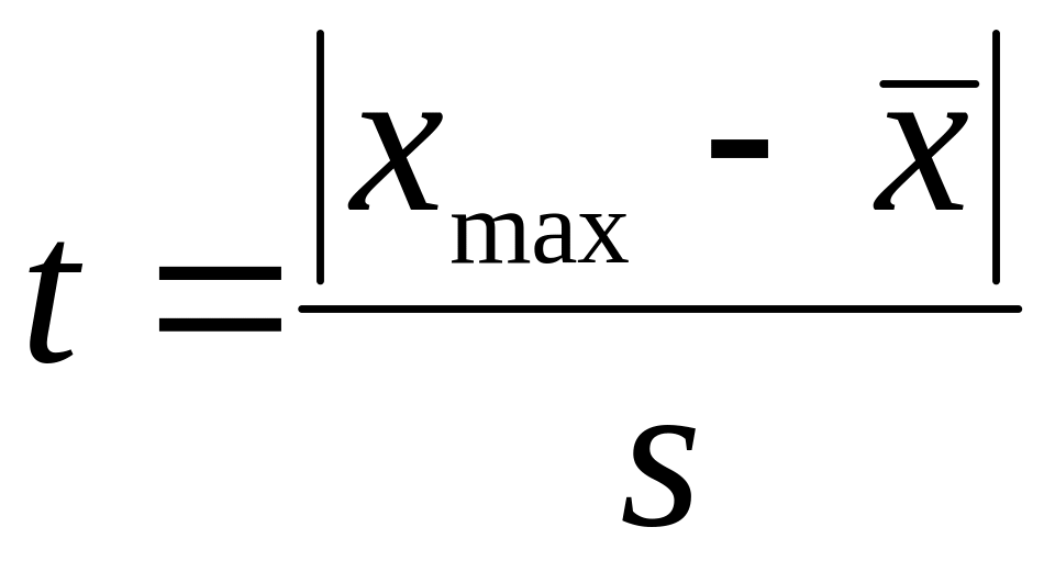
,
где

,

.
Для
проверки гипотезы о грубой ошибке
задается α – уровень значимости,
определяющий вероятность практически
невозможного события
P(t
ta)=
α,
состоящего
в том, что t
– реализация статистики превысит
критическое значение ta
.
Значение
величины ta
определяется по таблице приложения 10
по объему выборки n
и
уровню значимости α. Например, для
объема выборки
n
=
50 и уровня значимости α
=
0,05, значение ta=2,987.
Затем
вычисляются значения величин x*min
=
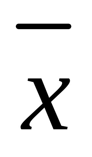
—
sta
и
x*max
=
+
sta.
Если xmin

x*min
,
или xmax
x*max
то
xmin
и
xmax
не являются грубыми ошибками. В
противоположном случае они являются
грубыми ошибками и исключаются из
выборки.
2.1.4. Построение статистических оценок математического ожидания и дисперсии
Статистические
оценки математического ожидания и
дисперсии разделяют на точечные и
интервальные (доверительные).
Построение точечных оценок
Математическим
ожиданием
M[X]
дискретной случайной величины X
называется сумма произведений всех
возможных значений случайной величины

на вероятности

этих значений:
M[X]
=

Дисперсией
случайной
величины называется математическое
ожидание квадрата соответствующей
центрированной случайной величины:
D[X]
= M[(X—
M[X])
]
=
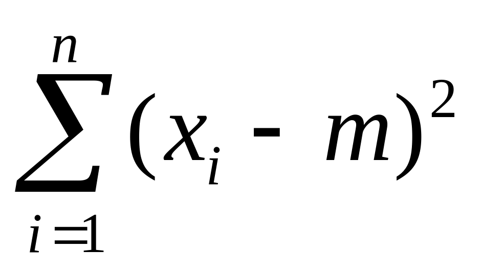
p
.
Статистической
оценкой а*
неизвестного параметра а
теоретического распределения называют
функцию от случайной выборки g(X1,
X2,
…, Xn).
Точечной
оценкой неизвестного параметра а
называют статистическую оценку,
реализация которой определяется одним
числом a*=
g(x1,
x2,
…, xn),
где x1,
x2,
…, xn
–
выборка измерений, т.е. результаты n
измерений случайной величины Х.
Реализация
точечной оценки математического ожидания
СВ определяется по формуле:
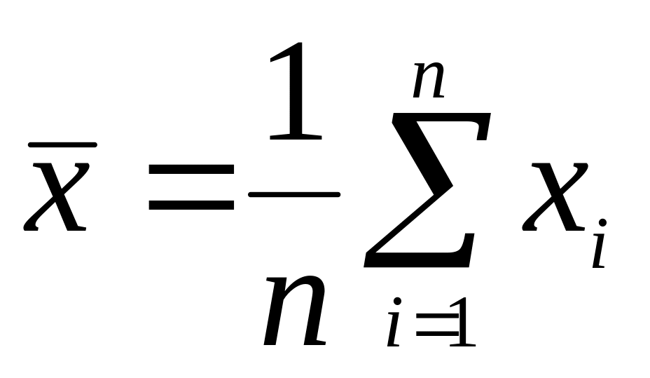
,
где

объем выборки
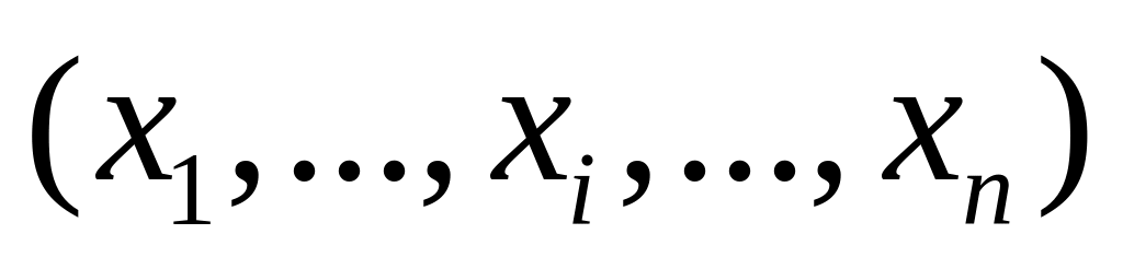
.
В
том случае, когда математическое ожидание
известно, реализация точечной оценки
дисперсии СВ определяется по формуле:

=
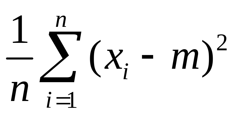
.
Если
математическое ожидание
неизвестно, то в качестве математического
ожидания определяется его оценка

.
В
этом случае, реализация точечной оценки
дисперсии СВ определяется по формуле:
=

.
Выборочная
дисперсия характеризует рассеяние
наблюдаемых значений выборки около
среднего значения

.
Соседние файлы в предмете [НЕСОРТИРОВАННОЕ]
- #
- #
- #
- #
- #
- #
- #
- #
- #
- #
- #
Памятка эксперту «Классификация ошибок»
К 7. Орфографические ошибки
Орфографические ошибки- неправильное написание слова, допущенное на письме, обычно в слабой фонетической позиции.
Однотипные и неоднотипные орфографические ошибки:
-
Однотипные- ошибки на одно и то же орфографическое правило. Эти ошибки исправляются, но при подсчете общего количества допущенных ошибок считаются 3 за 1, каждая последующая считается самостоятельной ошибкой. Примечание: не считаются однотипными ошибки, допущенные в словах с проверяемыми гласными в корне слова.
-
Повторяющиеся- ошибки в одном и том же повторяющемся слове или в корне однокоренных слов. Эти ошибки также считаются за одну.
Грубые и негрубые орфографические ошибки:
К негрубым орфографическим ошибкам относятся:
-
исключения из правил;
-
строчная и прописная буквы в собственных наименованиях;
-
не регулируемые правилами слитные и раздельные написания наречий;
-
слитное и раздельное написание НЕ с прилагательными и причастиями, выступающими в роли сказуемых;
-
различение НЕ и Ни в оборотах никто иной не…, ничто иное не…, не кто иной, как…, не что иное, как…, а также во фразах типа: Куда только он не обращался! Куда только он ни обращался, никто не мог дать ему ответ;
-
написание собственных имен нерусского происхождения;
-
написание И и Ы после приставок.
Другие виды ошибок:
-
Графические ошибки ( пи проверке не учитываются)- разновидность ошибок, связанных с графикой ( различные приемы сокращения слов, использование пробелов между словами, различные подчеркивания, шрифтовые выделения).
-
Описки-ошибки, вызванные невнимательностью пишущего или поспешностью написания. Они исправляются, но не выносятся на поля и не учитываются при подсчете ошибок. К опискам относятся:
-
пропуски букв;
-
перестановка букв;
-
замена одних букв другими;
-
добавление лишних букв.
К 8. Пунктуационные ошибки
Пунктуационные ошибки-ошибки, связанные с нарушением пунктуационных правил. 2 негрубые пунктуационные ошибки считаются за 1.
К негрубым пунктуационным ошибкам относятся :
-
употребление одного знака препинания вместо другого;
-
пропуск одного из двойных знаков препинания;
-
нарушение последовательности сочетающихся знаков или пропуск одного из сочетающихся знаков;
-
не относится к ошибкам авторская пунктуация.
Понятие об однотипных ошибках НЕ распространяется на пунктуационные ошибки.
К 9. Классификация грамматических ошибок
-
ошибки в образовании слов, связанных с нарушением словообразовательных форм;
-
ошибки в образовании форм различных частей речи, связанные с нарушением морфологических норм;
-
ошибки в построении словосочетаний, связанные с нарушением синтаксических норм;
-
ошибки в построении простого предложения, связанные с нарушением синтаксических норм;
-
ошибки в построении сложного предложения, связанные с нарушением синтаксических норм.
|
|
|
1. |
Неправильное использование приставок: зафотографировали (вм. сфотографировали). |
|
2. |
Неправильное использование суффиксов: одеяло мокнуло ( вм. мокло). |
|
3. |
Ошибки при образовании сложных слов: полуумный (вм. полоумный). |
|
4. |
Неправильное образование формы И.п. мн.ч.: торта (вм. торты), договора (вм. договоры). |
|
5. |
Неправильная форма рода: лёгкая тюль (вм. лёгкий ). |
|
6. |
Неправильная форма числа: вышел на подмосток ( вм. на подмостки). |
|
7. |
Нарушение норм склонения иноязычных фамилий: Повесть Аркадия и Георгия Вайнер ( вм. Вайнеров). |
|
8. |
Неправильное образование формы Р.п. мн.ч.: Пять килограмм (вм. пять килограммов), много грузинов (вм. грузин), новыми дверями (вм. дверьми). |
|
9. |
Ошибки в категории одушевленных и неодушевленных существительных: Я забрал его ферзь (вм. ферьзя). |
|
10. |
Склонение несклоняемого существительного: Мы побывали на горном плате (вм. плато). |
|
11. |
Неверное образование форм кратких прилагательных: Вывод беспочвенен (лучше беспочвен), ему свойственен оптимизм ( вм. свойствен). |
|
12. |
Ошибки при образовании степеней сравнения: Самый талантливейший поэт ( вм. самый талантливый), более тяжелее (вм. более тяжело). |
|
13. |
Неправильное образование местоимений 3-го лица мн.ч.: ихний сын (вм. их). |
|
14. |
Ошибки в образовании личных форм глаголов: ветер колыхает листву ( вм. колышет). |
|
15 |
Ошибки в образовании повелительного наклонения: едь (вм. езжай), ляжь (вм. ляг). |
|
16. |
Неверное образование видовых форм: институт организовывает подготовительные курсы (вм. организует). |
|
17. |
Неправильное образование действительных и страдательных причастий: Изделия, выпускающиеся в России (вм. выпускаемые). |
|
18. |
Ошибки при образовании деепричастий: Пиша диктант, нужно быть внимательным (нет литературной формы деепричастия). |
|
19. |
Ошибки при образовании наречий ( использование разговорной формы вместо литературной): тута, здеся (вм. тут, здесь). |
|
|
|
1. |
Неправильное использование сказуемого при подлежащем, выраженном собирательными существительными: Стая лебедей летели (вм. летела). Большинство участников собрания проголосовали ( вм. проголосовало). |
|
2. |
Неправильное употребление числа сказуемого: Там жила бабушка и ее внук (вм. жили). |
|
3. |
Согласование обобщающего слова и однородных членов: На конференции выступили делегаты из следующих городов: Красноярск, Москва… (вм. Красноярска, Москвы). |
|
|
|
1. |
Употребление неверно выбранного падежа: Согласно приказа (вм. приказу), заведующий кафедры (вм. кафедрой). |
|
|
|
1. |
Личное местоимение дублирует подлежащее: Этот автор, он всегда ставит острые вопросы. |
|
2. |
Расположение слов в предложении, не соответствующее грамматическим нормам русского языка: Ученики четко должны усвоить понятия (вм. должны четко усвоить). |
|
|
|
1. |
Рассогласование времен: Учебник дает знания, научит выделять главное. (вм. дает, учит). |
|
2. |
Объединение в одном ряду однородных членов родовых и видовых понятий: Он принес плоскогубцы, инструменты, молоток и гвозди. |
|
3. |
Парное сочетание несопоставимых понятий : Родители и друзья, коллеги и дети. |
|
4. |
Не сочетаемость опорного слова и одного из компонентов однородных членов: Проявление заботы и помощи радовали всех (нельзя проявлять помощь). |
|
5. |
Объединение в качестве однородных полных и кратких форм прилагательных: Комната просторная и светла (вм. просторна и светла). |
|
|
|
1. |
Употребление противительных союзов вместо соединительных: Тигр вскочил на спину слона, но задел лапами дрова, но дрова упали на него. |
|
2. |
Употребление лишнего союза: Онегин знал об этом, но однако ничего не предпринял. |
|
|
|
1. |
Одновременное употребление подчинительных и сочинительных союзов: Как только перестал дождь, и мы отправились домой (вм. Как только перестал дождь, мы отправились домой). |
|
2. |
Пропуск указательного слова (неоправданный эллипсис): В армии Петя просился (?), где опаснее. |
|
3. |
Тавтологическое употребление союзов и союзных слов, нагромождение придаточных частей: Когда утром казаки встали, Тарас удивился, когда увидел, что среди казаков нет Андрия. |
-
При вынесении грамматической ошибки эксперту необходимо делать на полях работы выпускника подробную запись, например: Г VII . 3
К 9. Классификация речевых ошибок
|
|
|
|
|
по значению слов. |
|
|
|
Следует сказать следующее. |
А. Блок-мастер звукозаписи. |
-
При вынесении речевой ошибки эксперту необходимо делать на полях работы выпускника подробную запись, например: Р2
Классификация фактических ошибок
|
Ф1. Искажение содержания литературного произведения, неправильное токование, неудачный подбор примеров: Счастьем для Обломова было одиночество и равнодушие. Ленский вернулся в свое имение из Англии. Базаров был нигилист и поэтому убил старуху топором. |
|
Ф2. Неточность в цитате, отсутствие указания на автора цитаты. Неверно названный автор цитаты: Книги много значат для меня, ведь еще Ленин сказал: «Век живи-век учись!» |
|
Ф3. Незнание исторических и др. фактов, в том числе, временное смешение: Великая Отечественная война 1812 года. Столица США-Нью-Йорк. |
|
Ф4 Неточности в именах и фамилиях, прозвищах литературных героев. Искажения в названиях литературных произведений, их жанров: Тургеньев, «Тарас и Бульба», в повести Тургенева «Преступление и наказание». |
-
При вынесении фактической ошибки эксперту необходимо делать на полях работы выпускника подробную запись, например: Ф2
Этические ошибки:
|
Речевая некорректность. Проявление речевой агрессии: грубое, оскорбительное высказывание; словесное выражение негативных эмоций, чувств или намерений в неприемлемой в данной речевой ситуации форме; угроза, грубое требование, обвинение, насмешка; употребление бранных слов, вульгаризмов, жаргонизмов, арго; высказывания, унижающие человеческое достоинство, выражающее высокомерие и циничное отношение к человеческой личности. |
Мне хотелось бы сделать автору замечание за его неумение передавать свои мысли. Этот текст меня бесит. Это старье, именуемое классикой. |
Логические ошибки
|
Л1. Сопоставление (противопоставление) двух логически неоднородных (различных по объему и по содержанию) понятий в предложении, тексте. |
На уроке присутствовали директор, библиотекарь, а также Анна Петровна и Зоя Ивановна Петрова. Он облокотился спиною на батарею. |
|
Л2.Нарушение причинно-следственных отношений. |
В последние годы очень много сделано для модернизации образования, однако педагоги работают по-старому, так как вопросы модернизации решаются слабо. |
|
Л3. Пропуск звена в объяснении, «логический скачок». |
Людской поток через наш двор перекрыть вряд ли возможно. (?)А как хочется, чтобы двор был украшением школы. |
|
Л4. Перестановка частей текста (если она не обусловлена заданием к сочинению или изложению). |
Пора вернуть этому слову его истинный смысл! Честь… Но как это сделать? |
|
Л5. Неоправданная подмена лица, от которого ведется повествование (например, сначала от первого, затем от третьего лица). |
Автор пишет о природе, описывает природу севера, вижу снега и просторы равнин. |
|
Л6.Сопоставление логически несопоставимых понятий. |
Синтаксис энциклопедических статей отличен от других научных статей. |
|
Композиционно-текстовые ошибки |
|
|
Л7.Неудачный зачин. |
В этом тексте автор… (указание на предыдущий контекст с помощью указательных словоформ). |
|
Л8. Ошибка в основной части:
|
|
|
Л9. Неудачная концовка: дублирование вывода, неоправданное повторение высказанной ранее мысли. |
-
При вынесении логической ошибки эксперту необходимо делать на полях работы выпускника подробную запись, например: Л2
10
При проверке и оценке экзаменационных работ учитывается грамотность выпускника. Приведенный ниже материал поможет при квалификации разных типов ошибок. А умение распознать ошибки поможет научиться не допускать их. Также очень важно знать, что такое грубые, негрубые, повторяющиеся ошибки, поскольку количество баллов напрямую зависит от типа ошибки.
Из критериев 7 и 8 в 2023 году исключили понятие «негрубой ошибки». Это значит, что негрубые ошибки вообще не будут учитываться. Учитываются только ГРУБЫЕ. Положение о повторяющихся, однотипных ошибках сохраняется и учитывается при оценивании сочинения. Также сохраняется положение об ошибках, которые не учитываются при проверке.
Орфографическая ошибка – это неправильное написание слова; она может быть допущена только на письме, обычно в слабой фонетической позиции (для гласных – в безударном положении, для согласных – на конце слова или перед другим согласным) или в слитно-раздельно-дефисных написаниях, например: на площаде, о синим карандаше, небыл, кто то, полапельсина.
1) в исключениях из правил;
2) в написании большой буквы в составных собственных наименованиях;
3) в случаях раздельного и слитного написания не с прилагательными ипричастиями, выступающими в роли сказуемого;
4) в написании -и -ы после приставок;
5) в трудных случаях различения не и ни (Куда он только не обращался!Куда он ни обращался, никто не мог дать ему ответ. Никто иной не …; не кто иной, как …; ничто иное не …; не что иное, как … и др.).
Каждая негрубая ошибка в 2022 г. оценивалась в 0,5 баллов, в 2023 негрубые ошибки не учитываются при проверке.
Повторяющаяся ошибка — ошибка, которая повторяется в одном и том же слове или в корне однокоренных слов (считается за 1 ошибку).
Однотипная ошибка на одно правило, если условия выбора правильного написания заключены в грамматических (в армии, в роще; колют, борются) и фонетических (пирожок, сверчок) особенностях данного слова.
Не считаются однотипными ошибки на такое правило, в котором для выяснения правильного написания одного слова требуется подобрать другое (опорное) слово или его форму (вода – воды, рот – ротик, грустный – грустить, резкий – резок).
Первые три однотипные ошибки считаются за одну ошибку, каждая следующая подобная ошибка учитывается как самостоятельная. Если в одном непроверяемом слове допущены две и более ошибки, то все они считаются за одну ошибку.
При оценке сочинения исправляются, но не учитываются следующие ошибки:
1. В переносе слов.
2. Буквы э/е после согласных в иноязычных словах (рэкет, пленэр) и после гласных в собственных именах (Мариетта).
3. В названиях, связанных с религией: М (м)асленица, Р (р)ождество, Б (б)ог.
4. При переносном употреблении собственных имен (Обломовы и обломовы).
5. В собственных именах нерусского происхождения; написание фамилий с первыми частями дон, ван, сент… (дон Педро и Дон Кихот).
6. Сложные существительные без соединительной гласной (в основном заимствования), не регулируемые правилами и не входящие в словарь- минимум (ленд-лиз, люля-кебаб, ноу-хау, папье-маше, перекати-поле, гуляй- город пресс-папье, но бефстроганов, метрдотель, портшез, прейскурант).
7. На правила, которые не включены в школьную программу (например, правило слитного / раздельного написания наречных единиц / наречий с приставкой / предлогом, например: в разлив, за глаза ругать, под стать, в бегах, в рассрочку, на попятную, в диковинку, на ощупь, на подхвате, на попа ставить (ср. действующее написание напропалую, врассыпную).
В отдельную категорию выделяются графические ошибки, т.е. различные описки, вызванные невнимательностью пишущего или поспешностью написания. Например, неправильные написания, искажающие звуковой облик слова (рапотает вместо работает, мемля вместо земля). Эти ошибки связаны с графикой, т.е. средствами письменности данного языка, фиксирующими отношения между буквами на письме и звуками устной речи. К графическим средствам помимо букв относятся различные приемы сокращения слов, использование пробелов между словами, различные подчеркивания и шрифтовые выделения.
Одиночные графические ошибки НЕ УЧИТЫВАЮТСЯ при проверке, но если таких ошибок больше 5 на 100 слов, то работу следует признать безграмотной.
*При оценке грамотности следует учитывать специфику письменной речи глухих и слабослышащих обучающихся, проявляющуюся в «аграмматизмах», (опускании предлогов, неправильном согласовании слов в роде, числе, «телеграфный стиль» и пр.), которые должны рассматриваться как однотипные ошибки.
Пунктуационная ошибка – это неиспользование пишущим необходимого знака препинания или его употребление там, где он не требуется, а также необоснованная замена одного знака препинания другим.
В соответствии с «Нормами оценки знаний, умений и навыков по русскому языку» исправляются, но не учитываются следующие пунктуационные ошибки:
1) тире в неполном предложении;
2)обособление несогласованных определений, относящихся к нарицательным именам существительным;
3) запятые при ограничительно-выделительных оборотах;
4) различение омонимичных частиц и междометий и, соответственно, невыделение или выделение их запятыми;
5) в передаче авторской пунктуации.
Среди пунктуационных ошибок следует выделять негрубые, которые ранее оценивали в
С 2023 года негрубые пунктуационные ошибки приравниваются к грубым.
1) в случаях, когда вместо одного знака препинания поставлен другой;
2) в пропуске одного из сочетающихся знаков препинания или в нарушении их последовательности.
Правила подсчета однотипных и повторяющихся ошибок на пунктуацию не распространяется.
Грамматическая ошибка – это ошибка в структуре языковой единицы: в структуре слова, словосочетания или предложения; это нарушение какой-либо грамматической нормы – словообразовательной, морфологической, синтаксической. Для обнаружения грамматической ошибки не нужен контекст, и в этом ее отличие от ошибки речевой, которая выявляется в контексте. Не следует также смешивать ошибки грамматические и орфографические.
Грамматические ошибки состоят:
- в ошибочном словообразовании (нарушении структуры слова);
- ошибочном образовании форм частей речи;
- в нарушении согласования, управления, видо-временной соотнесенности глагольных форм, неправильном употреблении предлогов;
- в нарушении связи между подлежащим и сказуемым;
- ошибочном построении предложения с деепричастным или причастным оборотом, однородными членами, а также сложных предложений
- в смешении прямой и косвенной речи;
- в нарушении границ предложения и др.
Примеры:
- подскользнуться вместо поскользнуться, благородность вместо благородство (здесь допущена ошибка в словообразовательной структуре слова, использована не та приставка или не тот суффикс);
- без комментарий вместо без комментариев, едь вместо поезжай, более легче (неправильно образована форма слова, т.е. нарушена морфологическая норма);
- заплатить за квартплату, удостоен наградой (нарушена структура словосочетания: не соблюдаются нормы управления);
- Покатавшись на катке, болят ноги; В сочинении я хотел показать значение спорта и почему я его люблю (неправильно построены предложения с деепричастным оборотом (1) и с однородными членами (2), т.е. нарушены синтаксические нормы).
Наиболее типичные морфологические и словообразовательные ошибки:
1) ошибки в образовании личных форм глаголов: Им двигает чувство сострадания (норма для употребленного в тексте значения глагола движет);
2) неправильное употребление временных форм глаголов: Эта книга дает знания об истории календаря, научит делать календарные расчеты быстро и точно (следует …даст.., научит… или …дает…, учит…);
3) ошибки в употреблении действительных и страдательных причастий: Ручейки воды, стекаемые вниз, поразили автора текста (следует стекавшие);
4) ошибки в образовании деепричастий: Вышев на сцену, певцы поклонились (норма выйдя);
5) неправильное образование наречий: Автор тута был не прав (норма тут);
6) ошибки, связанные с нарушением закономерностей и правил грамматики, возникающие под влиянием просторечия и диалектов.
Наиболее типичные синтаксические ошибки:
1) нарушение связи между подлежащим и сказуемым: Главное, чему теперь я хочу уделить внимание, это художественной стороне произведения (правильно это художественная сторона произведения); Чтобы приносить пользу Родине, нужно смелость, знания, честность (вместо нужны смелость, знания, честность);
2) ошибки, связанные с употреблением частиц: Хорошо было бы, если бы на картине стояла бы подпись художника; отрыв частицы от того компонента предложения, к которому она относится (обычно частицы ставятся перед теми членами предложения, которые они должны выделять, но эта закономерность часто нарушается в сочинениях): В тексте всего раскрываются две проблемы (ограничительная частица всего должна стоять перед подлежащим: … всего две проблемы);
3) неоправданный пропуск подлежащего (эллипсис): Его храбрость, (?) постоять за честь и справедливость привлекают автора текста;
4) неправильное построение сложносочиненного предложения: Ум автор текста понимает не только как просвещенность, интеллигентность, но и с понятием «умный» связывалось представление о вольнодумстве.
Речевая (в том числе стилистическая) ошибка – это ошибка не в построении, не в структуре языковой единицы, а в ее использовании, чаще всего в употреблении слова. По преимуществу это нарушения лексических норм, например: Штольц – один из главных героев одноименного романа Гончарова «Обломов»; Они потеряли на войне двух единственных сыновей. Само по себе слово одноименный (или единственный) ошибки не содержит, оно лишь неудачно употреблено, не «вписывается» в контекст, не сочетается по смыслу со своим ближайшим окружением.
К основным речевым (в том числе стилистическим) ошибкам следует относить:
1) употребление слова в несвойственном ему значении;
2) употребление иностилевых слов и выражений;
3) неуместное использование экспрессивных, эмоционально окрашенных средств;
4) немотивированное применение диалектных и просторечных слов и выражений, жаргонизмом
5) смешение лексики разных исторических эпох;
6) нарушение лексической сочетаемости (слова в русском языке сочетаются друг с другом в зависимости от их смысла; от традиций употребления, вызванных языковой практикой (слова с ограниченной сочетаемостью);
7) неразличение (смешение) паронимов;
8) употребление лишнего слова (плеоназм);
9) повторение или двойное употребление в словесном тексте близких по смыслу синонимов без оправданной необходимости (тавтология);
10) необоснованный пропуск слова;
11) бедность и однообразие синтаксических конструкций;
12) порядок слов, приводящий к неоднозначному пониманию предложения.
13) ошибки в употреблении синонимов, антонимов и др.
14) не устраненная контекстом многозначность.
Разграничение видов речевых (в том числе стилистических) ошибок особенно важно при оценивании работ отличного и хорошего уровня. В то же время следует помнить, что соблюдение единства стиля – самое высокое достижение пишущего. Поэтому отдельные стилистические погрешности, допущенные школьниками, предлагается считать стилистическими недочетами.
Речевые ошибки следует отличать от ошибок грамматических (об этом см. далее).
1. Неразличение (смешение) паронимов: Хищное (вместо хищническое) истребление лесов привело к образованию оврагов; В конце собрания слово представили (вместо предоставили) известному ученому; В таких случаях я взглядываю в «Философский словарь» (глагол взглянуть обычно имеет при себе дополнение с предлогом на: взглянуть на кого-нибудь или на что-нибудь, а глагол заглянуть, который необходимо употребить в этом предложении, имеет дополнение с предлогом в).
2. Ошибки в выборе синонима: Имя этого поэта знакомо во многих странах (вместо слова известно в предложении ошибочно употреблен его синоним знакомо); Теперь в нашей печати отводится значительное пространство для рекламы, и это нам не импонирует (в данном случае вместо слова пространство лучше употребить его синоним место; иноязычное слово импонирует также требует синонимической замены).
3. Ошибки при употреблении антонимов в построении антитезы: В третьей части текста не веселый, но и не мажорный мотив заставляет нас задуматься (антитеза требует четкости и точности в сопоставлении контрастных слов, а не веселый и мажорный не являются даже контекстуальными антонимами, поскольку не выражают разнополярных проявлений одного и того же признака).
4. Нарушение лексической сочетаемости: В этом книжном магазине очень дешевые цены; Леонид вперед меня выполнил задание; Узнав об аварии, начальник скоропостижно прибыл на объект.
ЭТИКО-РЕЧЕВЫЕ ОШИБКИ – это нарушения этических, в частности, этикетных норм при построении устной или письменной речи (монолога или диалога). Этико-речевые нормы, в свою очередь, входят в понятие риторического (речевого) идеала, представления о котором извлекаются из национальной философии, национальных речевых традиций, а также из универсальных (общечеловеческих) постулатов речевого общения и правил речевого этикета.
Этические ошибки совершаются тогда, когда говорящий или пишущий игнорирует этико-эстетический компонент речевой культуры, который в русской речевой традиции «подразумевает особую роль категорий гармонии, кротости, смирения, миролюбия, негневливости, уравновешенности, радости, а реализуется в диалогическом гармонизирующем воздействии, риторических принципах немногословия, спокойствия, правдивости, искренности, благожелательности, ритмической мерности, отказе от крика, клеветы, сплетни, осуждения ближнего» (Михальская А.К., 1996. С. 400).
Чтобы не нарушать этические нормы следует отказаться от:
- речевой агрессии, навешивания «ярлыков»
- инвективы (ругательств)
- жаргона и вульгаризмов
Важно помнить о том, что с этической точки зрения недопустимы никакие высказывания, унижающие человеческое достоинство, выражающие высокомерное и тем более циничное отношение к человеческой личности, его национальной принадлежности, культуре, религии и т.д. Подбирая слова, следует также помнить и об этикетных формулах.
На уровень этичности общения оказывают существенное влияние не только коммуникативная компетентность общающихся, но и их личностные качества. Этические нормы нарушают чаще всего люди, которым свойственны вспыльчивость, раздражительность, пристрастность, придирчивость, высокомерие, пренебрежительность, эгоцентризм и некоторые другие негативные качества. Тем не менее критическое отношение к своим речевым поступкам, самоконтроль и самодисциплина дают возможность минимизировать их отрицательное воздействие на культуру общения.
Это разновидность неязыковых ошибок, заключающаяся в том, что говорящий или пишущий, недостаточно хорошо владея информацией по обсуждаемой теме, приводит факты, противоречащие действительности, например: «Ленский вернулся в свое имение из Англии». Фактическая ошибка может состоять не только в полном искажении (подмене) факта, но и в его преувеличении или преуменьшении, напр.:«Маяковский – вдохновитель народа в борьбе с интервенцией»;
Фактические ошибки отражают низкий уровень знаний, поэтому работа по исправлению и предупреждению ошибок такого рода связана с повышением интеллектуального и культурного уровня. Говорящий или пишущий в своих рассуждениях должен использовать только достоверную информацию.
- Если в работе допущена одна негрубая фактическая ошибка, не связанная с пониманием проблемы исходного текста, то по критерию К12 выставляется 1 балл.
- Если негрубая фактическая ошибка повторяется в работе экзаменуемого, то она считается за 0,5 ошибки.
Грубой фактической ошибкой считается искажение авторской позиции и концепции автора произведения, привлекаемого в обосновании, а также вопиющие случаи неразличения автора-рассказчика-повествователя. (Раскольников на преступление идёт неосознанно; Лермонтов написал Евгения Онегина); (Чехов говорит Юлии Васильевне. А.П. Чехов «Размазня» ; Автор лежал возле взорванного поезда. В. Каверин «Два капитана»)
Необходимо различать фактические ошибки по К2 и по К12:если при комментировании допущена ошибка, связанная с пониманием проблема, то балл снимают за К2. Если допущена фактическая ошибка, связанная с содержанием текста или фоновыми знаниями, то снимается балл за К12.
Как правило, не учитываются фактические ошибки, связанные с деталями: несущественные искажения указаний на время, место, порядок действий персонажей и т. п. в привлекаемых для обоснования произведениях.
Вернуться в раздел СОЧИНЕНИЕ ЕГЭ
Industrial process data validation and reconciliation, or more briefly, process data reconciliation (PDR), is a technology that uses process information and mathematical methods in order to automatically ensure data validation and reconciliation by correcting measurements in industrial processes. The use of PDR allows for extracting accurate and reliable information about the state of industry processes from raw measurement data and produces a single consistent set of data representing the most likely process operation.
Models, data and measurement errors[edit]
Industrial processes, for example chemical or thermodynamic processes in chemical plants, refineries, oil or gas production sites, or power plants, are often represented by two fundamental means:
- Models that express the general structure of the processes,
- Data that reflects the state of the processes at a given point in time.
Models can have different levels of detail, for example one can incorporate simple mass or compound conservation balances, or more advanced thermodynamic models including energy conservation laws. Mathematically the model can be expressed by a nonlinear system of equations 

Error types[edit]
- Random and systematic errors
-

Normally distributed measurements without bias.
-

Normally distributed measurements with bias.
Data originates typically from measurements taken at different places throughout the industrial site, for example temperature, pressure, volumetric flow rate measurements etc. To understand the basic principles of PDR, it is important to first recognize that plant measurements are never 100% correct, i.e. raw measurement 

- random errors due to intrinsic sensor accuracy and
- systematic errors (or gross errors) due to sensor calibration or faulty data transmission.
Random errors means that the measurement 


Other sources of errors when calculating plant balances include process faults such as leaks, unmodeled heat losses, incorrect physical properties or other physical parameters used in equations, and incorrect structure such as unmodeled bypass lines. Other errors include unmodeled plant dynamics such as holdup changes, and other instabilities in plant operations that violate steady state (algebraic) models. Additional dynamic errors arise when measurements and samples are not taken at the same time, especially lab analyses.
The normal practice of using time averages for the data input partly reduces the dynamic problems. However, that does not completely resolve timing inconsistencies for infrequently-sampled data like lab analyses.
This use of average values, like a moving average, acts as a low-pass filter, so high frequency noise is mostly eliminated. The result is that, in practice, data reconciliation is mainly making adjustments to correct systematic errors like biases.
Necessity of removing measurement errors[edit]
ISA-95 is the international standard for the integration of enterprise and control systems[1] It asserts that:
Data reconciliation is a serious issue for enterprise-control integration. The data have to be valid to be useful for the enterprise system. The data must often be determined from physical measurements that have associated error factors. This must usually be converted into exact values for the enterprise system. This conversion may require manual, or intelligent reconciliation of the converted values […].
Systems must be set up to ensure that accurate data are sent to production and from production. Inadvertent operator or clerical errors may result in too much production, too little production, the wrong production, incorrect inventory, or missing inventory.
History[edit]
PDR has become more and more important due to industrial processes that are becoming more and more complex. PDR started in the early 1960s with applications aiming at closing material balances in production processes where raw measurements were available for all variables.[2] At the same time the problem of gross error identification and elimination has been presented.[3] In the late 1960s and 1970s unmeasured variables were taken into account in the data reconciliation process.,[4][5] PDR also became more mature by considering general nonlinear equation systems coming from thermodynamic models.,[6]
,[7][8] Quasi steady state dynamics for filtering and simultaneous parameter estimation over time were introduced in 1977 by Stanley and Mah.[7] Dynamic PDR was formulated as a nonlinear optimization problem by Liebman et al. in 1992.[9]
Data reconciliation[edit]
Data reconciliation is a technique that targets at correcting measurement errors that are due to measurement noise, i.e. random errors. From a statistical point of view the main assumption is that no systematic errors exist in the set of measurements, since they may bias the reconciliation results and reduce the robustness of the reconciliation.
Given 

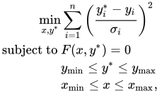
where




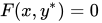


The term 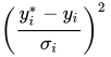
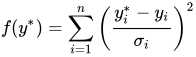
In other words, one wants to minimize the overall correction (measured in the least squares term) that is needed in order to satisfy the system constraints. Additionally, each least squares term is weighted by the standard deviation of the corresponding measurement. The standard deviation is related to the accuracy of the measurement. For example, at a 95% confidence level, the standard deviation is about half the accuracy.
Redundancy[edit]
- Sensor and topological redundancy
-
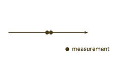
Sensor redundancy arising from multiple sensors of the same quantity at the same time at the same place.
Data reconciliation relies strongly on the concept of redundancy to correct the measurements as little as possible in order to satisfy the process constraints. Here, redundancy is defined differently from redundancy in information theory. Instead, redundancy arises from combining sensor data with the model (algebraic constraints), sometimes more specifically called «spatial redundancy»,[7] «analytical redundancy», or «topological redundancy».
Redundancy can be due to sensor redundancy, where sensors are duplicated in order to have more than one measurement of the same quantity. Redundancy also arises when a single variable can be estimated in several independent ways from separate sets of measurements at a given time or time averaging period, using the algebraic constraints.
Redundancy is linked to the concept of observability. A variable (or system) is observable if the models and sensor measurements can be used to uniquely determine its value (system state). A sensor is redundant if its removal causes no loss of observability. Rigorous definitions of observability, calculability, and redundancy, along with criteria for determining it, were established by Stanley and Mah,[10] for these cases with set constraints such as algebraic equations and inequalities. Next, we illustrate some special cases:
Topological redundancy is intimately linked with the degrees of freedom (

When speaking about topological redundancy we have to distinguish between measured and unmeasured variables. In the following let us denote by 

If the system 



i.e. the redundancy is the difference between the number of equations 

Simple counts of variables, equations, and measurements are inadequate for many systems, breaking down for several reasons: (a) Portions of a system might have redundancy, while others do not, and some portions might not even be possible to calculate, and (b) Nonlinearities can lead to different conclusions at different operating points. As an example, consider the following system with 4 streams and 2 units.
Example of calculable and non-calculable systems[edit]
We incorporate only flow conservation constraints and obtain 


If we have measurements for 


In 1981, observability and redundancy criteria were proven for these sorts of flow networks involving only mass and energy balance constraints.[12] After combining all the plant inputs and outputs into an «environment node», loss of observability corresponds to cycles of unmeasured streams. That is seen in the second case above, where streams a and b are in a cycle of unmeasured streams. Redundancy classification follows, by testing for a path of unmeasured streams, since that would lead to an unmeasured cycle if the measurement was removed. Measurements c and d are redundant in the second case above, even though part of the system is unobservable.
Benefits[edit]
Redundancy can be used as a source of information to cross-check and correct the measurements
Data validation[edit]
Data validation denotes all validation and verification actions before and after the reconciliation step.
Data filtering[edit]
Data filtering denotes the process of treating measured data such that the values become meaningful and lie within the range of expected values. Data filtering is necessary before the reconciliation process in order to increase robustness of the reconciliation step. There are several ways of data filtering, for example taking the average of several measured values over a well-defined time period.
Result validation[edit]
Result validation is the set of validation or verification actions taken after the reconciliation process and it takes into account measured and unmeasured variables as well as reconciled values. Result validation covers, but is not limited to, penalty analysis for determining the reliability of the reconciliation, or bound checks to ensure that the reconciled values lie in a certain range, e.g. the temperature has to be within some reasonable bounds.
Gross error detection[edit]
Result validation may include statistical tests to validate the reliability of the reconciled values, by checking whether gross errors exist in the set of measured values. These tests can be for example
- the chi square test (global test)
- the individual test.
If no gross errors exist in the set of measured values, then each penalty term in the objective function is a random variable that is normally distributed with mean equal to 0 and variance equal to 1. By consequence, the objective function is a random variable which follows a chi-square distribution, since it is the sum of the square of normally distributed random variables. Comparing the value of the objective function 


The individual test compares each penalty term in the objective function with the critical values of the normal distribution. If the
Advanced process data reconciliation[edit]
Advanced process data reconciliation (PDR) is an integrated approach of combining data reconciliation and data validation techniques, which is characterized by
- complex models incorporating besides mass balances also thermodynamics, momentum balances, equilibria constraints, hydrodynamics etc.
- gross error remediation techniques to ensure meaningfulness of the reconciled values,
- robust algorithms for solving the reconciliation problem.
Thermodynamic models[edit]
Simple models include mass balances only. When adding thermodynamic constraints such as energy balances to the model, its scope and the level of redundancy increases. Indeed, as we have seen above, the level of redundancy is defined as 

Gross error remediation[edit]

The workflow of an advanced data validation and reconciliation process.
Gross errors are measurement systematic errors that may bias the reconciliation results. Therefore, it is important to identify and eliminate these gross errors from the reconciliation process. After the reconciliation statistical tests can be applied that indicate whether or not a gross error does exist somewhere in the set of measurements. These techniques of gross error remediation are based on two concepts:
- gross error elimination
- gross error relaxation.
Gross error elimination determines one measurement that is biased by a systematic error and discards this measurement from the data set. The determination of the measurement to be discarded is based on different kinds of penalty terms that express how much the measured values deviate from the reconciled values. Once the gross errors are detected they are discarded from the measurements and the reconciliation can be done without these faulty measurements that spoil the reconciliation process. If needed, the elimination is repeated until no gross error exists in the set of measurements.
Gross error relaxation targets at relaxing the estimate for the uncertainty of suspicious measurements so that the reconciled value is in the 95% confidence interval. Relaxation typically finds application when it is not possible to determine which measurement around one unit is responsible for the gross error (equivalence of gross errors). Then measurement uncertainties of the measurements involved are increased.
It is important to note that the remediation of gross errors reduces the quality of the reconciliation, either the redundancy decreases (elimination) or the uncertainty of the measured data increases (relaxation). Therefore, it can only be applied when the initial level of redundancy is high enough to ensure that the data reconciliation can still be done (see Section 2,[11]).
Workflow[edit]
Advanced PDR solutions offer an integration of the techniques mentioned above:
- data acquisition from data historian, data base or manual inputs
- data validation and filtering of raw measurements
- data reconciliation of filtered measurements
- result verification
- range check
- gross error remediation (and go back to step 3)
- result storage (raw measurements together with reconciled values)
The result of an advanced PDR procedure is a coherent set of validated and reconciled process data.
Applications[edit]
PDR finds application mainly in industry sectors where either measurements are not accurate or even non-existing, like for example in the upstream sector where flow meters are difficult or expensive to position (see [13]); or where accurate data is of high importance, for example for security reasons in nuclear power plants (see [14]). Another field of application is performance and process monitoring (see [15]) in oil refining or in the chemical industry.
As PDR enables to calculate estimates even for unmeasured variables in a reliable way, the German Engineering Society (VDI Gesellschaft Energie und Umwelt) has accepted the technology of PDR as a means to replace expensive sensors in the nuclear power industry (see VDI norm 2048,[11]).
See also[edit]
- Process simulation
- Pinch analysis
- Industrial processes
- Chemical engineering
References[edit]
- ^ «ISA-95: the international standard for the integration of enterprise and control systems». isa-95.com.
- ^ D.R. Kuehn, H. Davidson, Computer Control II. Mathematics of Control, Chem. Eng. Process 57: 44–47, 1961.
- ^ V. Vaclavek, Studies on System Engineering I. On the Application of the Calculus of the Observations of Calculations of Chemical Engineering Balances, Coll. Czech Chem. Commun. 34: 3653, 1968.
- ^ V. Vaclavek, M. Loucka, Selection of Measurements Necessary to Achieve Multicomponent Mass Balances in Chemical Plant, Chem. Eng. Sci. 31: 1199–1205, 1976.
- ^ R.S.H. Mah, G.M. Stanley, D.W. Downing, Reconciliation and Rectification of Process Flow and Inventory Data, Ind. & Eng. Chem. Proc. Des. Dev. 15: 175–183, 1976.
- ^ J.C. Knepper, J.W. Gorman, Statistical Analysis of Constrained Data Sets, AiChE Journal 26: 260–164, 1961.
- ^ a b c G.M. Stanley and R.S.H. Mah, Estimation of Flows and Temperatures in Process Networks, AIChE Journal 23: 642–650, 1977.
- ^ P. Joris, B. Kalitventzeff, Process measurements analysis and validation, Proc. CEF’87: Use Comput. Chem. Eng., Italy, 41–46, 1987.
- ^ M.J. Liebman, T.F. Edgar, L.S. Lasdon, Efficient Data Reconciliation and Estimation for Dynamic Processes Using Nonlinear Programming Techniques, Computers Chem. Eng. 16: 963–986, 1992.
- ^
Stanley G.M. and Mah, R.S.H., «Observability and Redundancy in Process Data Estimation, Chem. Engng. Sci. 36, 259 (1981) - ^ a b c VDI-Gesellschaft Energie und Umwelt, «Guidelines — VDI 2048 Blatt 1 — “Control and quality improvement of process data and their uncertainties by means of correction calculation for operation and acceptance tests”; VDI 2048 Part 1; September 2017», Association of German Engineers, 2017.
- ^ Stanley G.M., and Mah R.S.H., «Observability and Redundancy Classification in Process Networks», Chem. Engng. Sci. 36, 1941 (1981)
- ^ P. Delava, E. Maréchal, B. Vrielynck, B. Kalitventzeff (1999), Modelling of a Crude Oil Distillation Unit in Term of Data Reconciliation with ASTM or TBP Curves as Direct Input – Application : Crude Oil Preheating Train, Proceedings of ESCAPE-9 conference, Budapest, May 31-June 2, 1999, supplementary volume, p. 17-20.
- ^ M. Langenstein, J. Jansky, B. Laipple (2004), Finding Megawatts in nuclear power plants with process data validation, Proceedings of ICONE12, Arlington, USA, April 25–29, 2004.
- ^ Th. Amand, G. Heyen, B. Kalitventzeff, Plant Monitoring and Fault Detection: Synergy between Data Reconciliation and Principal Component Analysis, Comp. and Chem, Eng. 25, p. 501-507, 2001.
- Alexander, Dave, Tannar, Dave & Wasik, Larry «Mill Information System uses Dynamic Data Reconciliation for Accurate Energy Accounting» TAPPI Fall Conference 2007.[1][permanent dead link]
- Rankin, J. & Wasik, L. «Dynamic Data Reconciliation of Batch Pulping Processes (for On-Line Prediction)» PAPTAC Spring Conference 2009.
- S. Narasimhan, C. Jordache, Data reconciliation and gross error detection: an intelligent use of process data, Golf Publishing Company, Houston, 2000.
- V. Veverka, F. Madron, ‘Material and Energy Balancing in the Process Industries, Elsevier Science BV, Amsterdam, 1997.
- J. Romagnoli, M.C. Sanchez, Data processing and reconciliation for chemical process operations, Academic Press, 2000.
Industrial process data validation and reconciliation, or more briefly, process data reconciliation (PDR), is a technology that uses process information and mathematical methods in order to automatically ensure data validation and reconciliation by correcting measurements in industrial processes. The use of PDR allows for extracting accurate and reliable information about the state of industry processes from raw measurement data and produces a single consistent set of data representing the most likely process operation.
Models, data and measurement errors[edit]
Industrial processes, for example chemical or thermodynamic processes in chemical plants, refineries, oil or gas production sites, or power plants, are often represented by two fundamental means:
- Models that express the general structure of the processes,
- Data that reflects the state of the processes at a given point in time.
Models can have different levels of detail, for example one can incorporate simple mass or compound conservation balances, or more advanced thermodynamic models including energy conservation laws. Mathematically the model can be expressed by a nonlinear system of equations
Error types[edit]
- Random and systematic errors
-
Normally distributed measurements without bias.
-
Normally distributed measurements with bias.
Data originates typically from measurements taken at different places throughout the industrial site, for example temperature, pressure, volumetric flow rate measurements etc. To understand the basic principles of PDR, it is important to first recognize that plant measurements are never 100% correct, i.e. raw measurement
- random errors due to intrinsic sensor accuracy and
- systematic errors (or gross errors) due to sensor calibration or faulty data transmission.
Random errors means that the measurement
Other sources of errors when calculating plant balances include process faults such as leaks, unmodeled heat losses, incorrect physical properties or other physical parameters used in equations, and incorrect structure such as unmodeled bypass lines. Other errors include unmodeled plant dynamics such as holdup changes, and other instabilities in plant operations that violate steady state (algebraic) models. Additional dynamic errors arise when measurements and samples are not taken at the same time, especially lab analyses.
The normal practice of using time averages for the data input partly reduces the dynamic problems. However, that does not completely resolve timing inconsistencies for infrequently-sampled data like lab analyses.
This use of average values, like a moving average, acts as a low-pass filter, so high frequency noise is mostly eliminated. The result is that, in practice, data reconciliation is mainly making adjustments to correct systematic errors like biases.
Necessity of removing measurement errors[edit]
ISA-95 is the international standard for the integration of enterprise and control systems[1] It asserts that:
Data reconciliation is a serious issue for enterprise-control integration. The data have to be valid to be useful for the enterprise system. The data must often be determined from physical measurements that have associated error factors. This must usually be converted into exact values for the enterprise system. This conversion may require manual, or intelligent reconciliation of the converted values […].
Systems must be set up to ensure that accurate data are sent to production and from production. Inadvertent operator or clerical errors may result in too much production, too little production, the wrong production, incorrect inventory, or missing inventory.
History[edit]
PDR has become more and more important due to industrial processes that are becoming more and more complex. PDR started in the early 1960s with applications aiming at closing material balances in production processes where raw measurements were available for all variables.[2] At the same time the problem of gross error identification and elimination has been presented.[3] In the late 1960s and 1970s unmeasured variables were taken into account in the data reconciliation process.,[4][5] PDR also became more mature by considering general nonlinear equation systems coming from thermodynamic models.,[6]
,[7][8] Quasi steady state dynamics for filtering and simultaneous parameter estimation over time were introduced in 1977 by Stanley and Mah.[7] Dynamic PDR was formulated as a nonlinear optimization problem by Liebman et al. in 1992.[9]
Data reconciliation[edit]
Data reconciliation is a technique that targets at correcting measurement errors that are due to measurement noise, i.e. random errors. From a statistical point of view the main assumption is that no systematic errors exist in the set of measurements, since they may bias the reconciliation results and reduce the robustness of the reconciliation.
Given
where
The term
In other words, one wants to minimize the overall correction (measured in the least squares term) that is needed in order to satisfy the system constraints. Additionally, each least squares term is weighted by the standard deviation of the corresponding measurement. The standard deviation is related to the accuracy of the measurement. For example, at a 95% confidence level, the standard deviation is about half the accuracy.
Redundancy[edit]
- Sensor and topological redundancy
-
Sensor redundancy arising from multiple sensors of the same quantity at the same time at the same place.
Data reconciliation relies strongly on the concept of redundancy to correct the measurements as little as possible in order to satisfy the process constraints. Here, redundancy is defined differently from redundancy in information theory. Instead, redundancy arises from combining sensor data with the model (algebraic constraints), sometimes more specifically called «spatial redundancy»,[7] «analytical redundancy», or «topological redundancy».
Redundancy can be due to sensor redundancy, where sensors are duplicated in order to have more than one measurement of the same quantity. Redundancy also arises when a single variable can be estimated in several independent ways from separate sets of measurements at a given time or time averaging period, using the algebraic constraints.
Redundancy is linked to the concept of observability. A variable (or system) is observable if the models and sensor measurements can be used to uniquely determine its value (system state). A sensor is redundant if its removal causes no loss of observability. Rigorous definitions of observability, calculability, and redundancy, along with criteria for determining it, were established by Stanley and Mah,[10] for these cases with set constraints such as algebraic equations and inequalities. Next, we illustrate some special cases:
Topological redundancy is intimately linked with the degrees of freedom (
When speaking about topological redundancy we have to distinguish between measured and unmeasured variables. In the following let us denote by
If the system
i.e. the redundancy is the difference between the number of equations
Simple counts of variables, equations, and measurements are inadequate for many systems, breaking down for several reasons: (a) Portions of a system might have redundancy, while others do not, and some portions might not even be possible to calculate, and (b) Nonlinearities can lead to different conclusions at different operating points. As an example, consider the following system with 4 streams and 2 units.
Example of calculable and non-calculable systems[edit]
We incorporate only flow conservation constraints and obtain
If we have measurements for
In 1981, observability and redundancy criteria were proven for these sorts of flow networks involving only mass and energy balance constraints.[12] After combining all the plant inputs and outputs into an «environment node», loss of observability corresponds to cycles of unmeasured streams. That is seen in the second case above, where streams a and b are in a cycle of unmeasured streams. Redundancy classification follows, by testing for a path of unmeasured streams, since that would lead to an unmeasured cycle if the measurement was removed. Measurements c and d are redundant in the second case above, even though part of the system is unobservable.
Benefits[edit]
Redundancy can be used as a source of information to cross-check and correct the measurements
Data validation[edit]
Data validation denotes all validation and verification actions before and after the reconciliation step.
Data filtering[edit]
Data filtering denotes the process of treating measured data such that the values become meaningful and lie within the range of expected values. Data filtering is necessary before the reconciliation process in order to increase robustness of the reconciliation step. There are several ways of data filtering, for example taking the average of several measured values over a well-defined time period.
Result validation[edit]
Result validation is the set of validation or verification actions taken after the reconciliation process and it takes into account measured and unmeasured variables as well as reconciled values. Result validation covers, but is not limited to, penalty analysis for determining the reliability of the reconciliation, or bound checks to ensure that the reconciled values lie in a certain range, e.g. the temperature has to be within some reasonable bounds.
Gross error detection[edit]
Result validation may include statistical tests to validate the reliability of the reconciled values, by checking whether gross errors exist in the set of measured values. These tests can be for example
- the chi square test (global test)
- the individual test.
If no gross errors exist in the set of measured values, then each penalty term in the objective function is a random variable that is normally distributed with mean equal to 0 and variance equal to 1. By consequence, the objective function is a random variable which follows a chi-square distribution, since it is the sum of the square of normally distributed random variables. Comparing the value of the objective function
The individual test compares each penalty term in the objective function with the critical values of the normal distribution. If the
Advanced process data reconciliation[edit]
Advanced process data reconciliation (PDR) is an integrated approach of combining data reconciliation and data validation techniques, which is characterized by
- complex models incorporating besides mass balances also thermodynamics, momentum balances, equilibria constraints, hydrodynamics etc.
- gross error remediation techniques to ensure meaningfulness of the reconciled values,
- robust algorithms for solving the reconciliation problem.
Thermodynamic models[edit]
Simple models include mass balances only. When adding thermodynamic constraints such as energy balances to the model, its scope and the level of redundancy increases. Indeed, as we have seen above, the level of redundancy is defined as
Gross error remediation[edit]
The workflow of an advanced data validation and reconciliation process.
Gross errors are measurement systematic errors that may bias the reconciliation results. Therefore, it is important to identify and eliminate these gross errors from the reconciliation process. After the reconciliation statistical tests can be applied that indicate whether or not a gross error does exist somewhere in the set of measurements. These techniques of gross error remediation are based on two concepts:
- gross error elimination
- gross error relaxation.
Gross error elimination determines one measurement that is biased by a systematic error and discards this measurement from the data set. The determination of the measurement to be discarded is based on different kinds of penalty terms that express how much the measured values deviate from the reconciled values. Once the gross errors are detected they are discarded from the measurements and the reconciliation can be done without these faulty measurements that spoil the reconciliation process. If needed, the elimination is repeated until no gross error exists in the set of measurements.
Gross error relaxation targets at relaxing the estimate for the uncertainty of suspicious measurements so that the reconciled value is in the 95% confidence interval. Relaxation typically finds application when it is not possible to determine which measurement around one unit is responsible for the gross error (equivalence of gross errors). Then measurement uncertainties of the measurements involved are increased.
It is important to note that the remediation of gross errors reduces the quality of the reconciliation, either the redundancy decreases (elimination) or the uncertainty of the measured data increases (relaxation). Therefore, it can only be applied when the initial level of redundancy is high enough to ensure that the data reconciliation can still be done (see Section 2,[11]).
Workflow[edit]
Advanced PDR solutions offer an integration of the techniques mentioned above:
- data acquisition from data historian, data base or manual inputs
- data validation and filtering of raw measurements
- data reconciliation of filtered measurements
- result verification
- range check
- gross error remediation (and go back to step 3)
- result storage (raw measurements together with reconciled values)
The result of an advanced PDR procedure is a coherent set of validated and reconciled process data.
Applications[edit]
PDR finds application mainly in industry sectors where either measurements are not accurate or even non-existing, like for example in the upstream sector where flow meters are difficult or expensive to position (see [13]); or where accurate data is of high importance, for example for security reasons in nuclear power plants (see [14]). Another field of application is performance and process monitoring (see [15]) in oil refining or in the chemical industry.
As PDR enables to calculate estimates even for unmeasured variables in a reliable way, the German Engineering Society (VDI Gesellschaft Energie und Umwelt) has accepted the technology of PDR as a means to replace expensive sensors in the nuclear power industry (see VDI norm 2048,[11]).
See also[edit]
- Process simulation
- Pinch analysis
- Industrial processes
- Chemical engineering
References[edit]
- ^ «ISA-95: the international standard for the integration of enterprise and control systems». isa-95.com.
- ^ D.R. Kuehn, H. Davidson, Computer Control II. Mathematics of Control, Chem. Eng. Process 57: 44–47, 1961.
- ^ V. Vaclavek, Studies on System Engineering I. On the Application of the Calculus of the Observations of Calculations of Chemical Engineering Balances, Coll. Czech Chem. Commun. 34: 3653, 1968.
- ^ V. Vaclavek, M. Loucka, Selection of Measurements Necessary to Achieve Multicomponent Mass Balances in Chemical Plant, Chem. Eng. Sci. 31: 1199–1205, 1976.
- ^ R.S.H. Mah, G.M. Stanley, D.W. Downing, Reconciliation and Rectification of Process Flow and Inventory Data, Ind. & Eng. Chem. Proc. Des. Dev. 15: 175–183, 1976.
- ^ J.C. Knepper, J.W. Gorman, Statistical Analysis of Constrained Data Sets, AiChE Journal 26: 260–164, 1961.
- ^ a b c G.M. Stanley and R.S.H. Mah, Estimation of Flows and Temperatures in Process Networks, AIChE Journal 23: 642–650, 1977.
- ^ P. Joris, B. Kalitventzeff, Process measurements analysis and validation, Proc. CEF’87: Use Comput. Chem. Eng., Italy, 41–46, 1987.
- ^ M.J. Liebman, T.F. Edgar, L.S. Lasdon, Efficient Data Reconciliation and Estimation for Dynamic Processes Using Nonlinear Programming Techniques, Computers Chem. Eng. 16: 963–986, 1992.
- ^
Stanley G.M. and Mah, R.S.H., «Observability and Redundancy in Process Data Estimation, Chem. Engng. Sci. 36, 259 (1981) - ^ a b c VDI-Gesellschaft Energie und Umwelt, «Guidelines — VDI 2048 Blatt 1 — “Control and quality improvement of process data and their uncertainties by means of correction calculation for operation and acceptance tests”; VDI 2048 Part 1; September 2017», Association of German Engineers, 2017.
- ^ Stanley G.M., and Mah R.S.H., «Observability and Redundancy Classification in Process Networks», Chem. Engng. Sci. 36, 1941 (1981)
- ^ P. Delava, E. Maréchal, B. Vrielynck, B. Kalitventzeff (1999), Modelling of a Crude Oil Distillation Unit in Term of Data Reconciliation with ASTM or TBP Curves as Direct Input – Application : Crude Oil Preheating Train, Proceedings of ESCAPE-9 conference, Budapest, May 31-June 2, 1999, supplementary volume, p. 17-20.
- ^ M. Langenstein, J. Jansky, B. Laipple (2004), Finding Megawatts in nuclear power plants with process data validation, Proceedings of ICONE12, Arlington, USA, April 25–29, 2004.
- ^ Th. Amand, G. Heyen, B. Kalitventzeff, Plant Monitoring and Fault Detection: Synergy between Data Reconciliation and Principal Component Analysis, Comp. and Chem, Eng. 25, p. 501-507, 2001.
- Alexander, Dave, Tannar, Dave & Wasik, Larry «Mill Information System uses Dynamic Data Reconciliation for Accurate Energy Accounting» TAPPI Fall Conference 2007.[1][permanent dead link]
- Rankin, J. & Wasik, L. «Dynamic Data Reconciliation of Batch Pulping Processes (for On-Line Prediction)» PAPTAC Spring Conference 2009.
- S. Narasimhan, C. Jordache, Data reconciliation and gross error detection: an intelligent use of process data, Golf Publishing Company, Houston, 2000.
- V. Veverka, F. Madron, ‘Material and Energy Balancing in the Process Industries, Elsevier Science BV, Amsterdam, 1997.
- J. Romagnoli, M.C. Sanchez, Data processing and reconciliation for chemical process operations, Academic Press, 2000.