Python is a great language for doing data analysis, primarily because of the fantastic ecosystem of data-centric Python packages. Pandas is one of those packages that makes importing and analyzing data much easier.
Analyzing data requires a lot of filtering operations. Pandas provide many methods to filter a Data frame and Dataframe.query() is one of them.
Syntax: DataFrame.query(expr, inplace=False, **kwargs)
Parameters:
expr: Expression in string form to filter data.
inplace: Make changes in the original data frame if True
kwargs: Other keyword arguments.Return type: Filtered Data frame
To download the CSV file used, Click Here.
Note: Dataframe.query() method only works if the column name doesn’t have any empty spaces. So before applying the method, spaces in column names are replaced with ‘_’
Example #1: Single condition filtering
In this example, the data is filtered on the basis of single condition. Before applying the query() method, the spaces in column names have been replaced with ‘_’.
import pandas as pd
data = pd.read_csv("employees.csv")
data.columns =[column.replace(" ", "_") for column in data.columns]
data.query('Senior_Management == True', inplace = True)
data
Output:
As shown in the output image, the data now only have rows where Senior Management is True.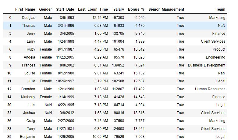
Example #2: Multiple condition filtering
In this example, dataframe has been filtered on multiple conditions. Before applying the query() method, the spaces in column names have been replaced with ‘_’.
import pandas as pd
data = pd.read_csv("employees.csv")
data.columns =[column.replace(" ", "_") for column in data.columns]
data.query('Senior_Management == True
and Gender =="Male" and Team =="Marketing"
and First_Name =="Johnny"', inplace = True)
data
Output:
As shown in the output image, only two rows have been returned on the basis of filters applied.
Python is a great language for doing data analysis, primarily because of the fantastic ecosystem of data-centric Python packages. Pandas is one of those packages that makes importing and analyzing data much easier.
Analyzing data requires a lot of filtering operations. Pandas provide many methods to filter a Data frame and Dataframe.query() is one of them.
Syntax: DataFrame.query(expr, inplace=False, **kwargs)
Parameters:
expr: Expression in string form to filter data.
inplace: Make changes in the original data frame if True
kwargs: Other keyword arguments.Return type: Filtered Data frame
To download the CSV file used, Click Here.
Note: Dataframe.query() method only works if the column name doesn’t have any empty spaces. So before applying the method, spaces in column names are replaced with ‘_’
Example #1: Single condition filtering
In this example, the data is filtered on the basis of single condition. Before applying the query() method, the spaces in column names have been replaced with ‘_’.
import pandas as pd
data = pd.read_csv("employees.csv")
data.columns =[column.replace(" ", "_") for column in data.columns]
data.query('Senior_Management == True', inplace = True)
data
Output:
As shown in the output image, the data now only have rows where Senior Management is True.
Example #2: Multiple condition filtering
In this example, dataframe has been filtered on multiple conditions. Before applying the query() method, the spaces in column names have been replaced with ‘_’.
import pandas as pd
data = pd.read_csv("employees.csv")
data.columns =[column.replace(" ", "_") for column in data.columns]
data.query('Senior_Management == True
and Gender =="Male" and Team =="Marketing"
and First_Name =="Johnny"', inplace = True)
data
Output:
As shown in the output image, only two rows have been returned on the basis of filters applied.
Python expressions lets us check for conditions and make decisions based on the result. It can let us check for various conditions like greater than, less than, equal to, not equal to, etc. We can check for conditions like the presence of variables in sequences or scalar values in sequences. We can even compare different variables using expressions and make decisions based on that. Python provides constructs like ‘>,<,>=,<=,=,!=,~, &, |,~’ etc for performing various conditions.
Pandas dataframes are the most commonly used data structure to store and manipulate tabular data in Python. What if we can use python expressions to filter rows of pandas dataframe. It can make code quite easy to understand if we can filter rows of pandas dataframe by providing python expressions specifying some conditions to filter rows.
To use python expressions with pandas dataframe, it provides a method named query() which takes as input python expression and filters rows of dataframe based on the condition specified through expression. The expression can use column names of pandas dataframe inside it and compare it against scalar, local variable, etc to make decisions. We need to provide expression as a string to query() method. The query() method used eval() method behind the scene to evaluate Python expressions.
As a part of this tutorial, we’ll explain how we can use Python expressions to filter rows of pandas dataframe using query() method. We have created many different examples to explain different conditions covering the majority of scenarios. For a few of our examples, we have also explained the second way of filtering rows without using query() method for comparison purposes.
Below we have imported pandas and numpy libraries that we’ll use in our tutorial.
import pandas as pd

print("Pandas Version : {}",format(pd.__version__))
Pandas Version : {} 1.3.4
In the below cell, we have created a sample dataframe that we’ll use to explain query() method. The index of the dataframe is the datetime index, five columns are random floats and one last column has categorical data.
np.random.seed(123)

data = np.random.rand(10,5)

df1 = pd.DataFrame(data=data, index=pd.date_range(start="2021-1-1", periods=10), columns=list("ABCDE"))

df1["Type"] = np.random.choice(["Class1", "Class2", "Class3"], size=10)

df1
| A | B | C | D | E | Type | |
|---|---|---|---|---|---|---|
| 2021-01-01 | 0.696469 | 0.286139 | 0.226851 | 0.551315 | 0.719469 | Class2 |
| 2021-01-02 | 0.423106 | 0.980764 | 0.684830 | 0.480932 | 0.392118 | Class1 |
| 2021-01-03 | 0.343178 | 0.729050 | 0.438572 | 0.059678 | 0.398044 | Class3 |
| 2021-01-04 | 0.737995 | 0.182492 | 0.175452 | 0.531551 | 0.531828 | Class2 |
| 2021-01-05 | 0.634401 | 0.849432 | 0.724455 | 0.611024 | 0.722443 | Class2 |
| 2021-01-06 | 0.322959 | 0.361789 | 0.228263 | 0.293714 | 0.630976 | Class1 |
| 2021-01-07 | 0.092105 | 0.433701 | 0.430863 | 0.493685 | 0.425830 | Class2 |
| 2021-01-08 | 0.312261 | 0.426351 | 0.893389 | 0.944160 | 0.501837 | Class2 |
| 2021-01-09 | 0.623953 | 0.115618 | 0.317285 | 0.414826 | 0.866309 | Class1 |
| 2021-01-10 | 0.250455 | 0.483034 | 0.985560 | 0.519485 | 0.612895 | Class1 |
Example 1
Our first example explains how we can include the simple expression to compare the value of a particular column against a scalar value and filter rows based on results. We have called query() method with expression ‘A > 0.5’ which will check each value of column ‘A’ and keep only entries which are greater than 5.
In the next cell after the below cell, we have explained how we can perform the same operation without using query() method.
| A | B | C | D | E | Type | |
|---|---|---|---|---|---|---|
| 2021-01-01 | 0.696469 | 0.286139 | 0.226851 | 0.551315 | 0.719469 | Class2 |
| 2021-01-04 | 0.737995 | 0.182492 | 0.175452 | 0.531551 | 0.531828 | Class2 |
| 2021-01-05 | 0.634401 | 0.849432 | 0.724455 | 0.611024 | 0.722443 | Class2 |
| 2021-01-09 | 0.623953 | 0.115618 | 0.317285 | 0.414826 | 0.866309 | Class1 |
| A | B | C | D | E | Type | |
|---|---|---|---|---|---|---|
| 2021-01-01 | 0.696469 | 0.286139 | 0.226851 | 0.551315 | 0.719469 | Class2 |
| 2021-01-04 | 0.737995 | 0.182492 | 0.175452 | 0.531551 | 0.531828 | Class2 |
| 2021-01-05 | 0.634401 | 0.849432 | 0.724455 | 0.611024 | 0.722443 | Class2 |
| 2021-01-09 | 0.623953 | 0.115618 | 0.317285 | 0.414826 | 0.866309 | Class1 |
Example 2
Below we have created another example explaining the usage of query() method. This time we have checked for condition ‘E * 10 > 5’ which will first multiply values of column ‘E’ by scalar 10 and then check which entries are greater than 5.
Then in the next cell after the below cell, we have explained how we can perform the same thing without using query() function.
| A | B | C | D | E | Type | |
|---|---|---|---|---|---|---|
| 2021-01-01 | 0.696469 | 0.286139 | 0.226851 | 0.551315 | 0.719469 | Class2 |
| 2021-01-04 | 0.737995 | 0.182492 | 0.175452 | 0.531551 | 0.531828 | Class2 |
| 2021-01-05 | 0.634401 | 0.849432 | 0.724455 | 0.611024 | 0.722443 | Class2 |
| 2021-01-06 | 0.322959 | 0.361789 | 0.228263 | 0.293714 | 0.630976 | Class1 |
| 2021-01-08 | 0.312261 | 0.426351 | 0.893389 | 0.944160 | 0.501837 | Class2 |
| 2021-01-09 | 0.623953 | 0.115618 | 0.317285 | 0.414826 | 0.866309 | Class1 |
| 2021-01-10 | 0.250455 | 0.483034 | 0.985560 | 0.519485 | 0.612895 | Class1 |
| A | B | C | D | E | Type | |
|---|---|---|---|---|---|---|
| 2021-01-01 | 0.696469 | 0.286139 | 0.226851 | 0.551315 | 0.719469 | Class2 |
| 2021-01-04 | 0.737995 | 0.182492 | 0.175452 | 0.531551 | 0.531828 | Class2 |
| 2021-01-05 | 0.634401 | 0.849432 | 0.724455 | 0.611024 | 0.722443 | Class2 |
| 2021-01-06 | 0.322959 | 0.361789 | 0.228263 | 0.293714 | 0.630976 | Class1 |
| 2021-01-08 | 0.312261 | 0.426351 | 0.893389 | 0.944160 | 0.501837 | Class2 |
| 2021-01-09 | 0.623953 | 0.115618 | 0.317285 | 0.414826 | 0.866309 | Class1 |
| 2021-01-10 | 0.250455 | 0.483034 | 0.985560 | 0.519485 | 0.612895 | Class1 |
Example 3
In this example, we are checking for condition ‘C — 0.5 > 0.4’ using query() function. We are subtracting scalar value 0.5 from each value of column ‘C’ and only keeping entries where values after subtraction are greater than 0.4.
Then in the next cell after the below cell, we have included code to do the same operation without using query() method.
| A | B | C | D | E | Type | |
|---|---|---|---|---|---|---|
| 2021-01-10 | 0.250455 | 0.483034 | 0.98556 | 0.519485 | 0.612895 | Class1 |
df1[(df1["C"] - 0.5) > 0.4]
| A | B | C | D | E | Type | |
|---|---|---|---|---|---|---|
| 2021-01-10 | 0.250455 | 0.483034 | 0.98556 | 0.519485 | 0.612895 | Class1 |
Example 4
In this example, we are checking for condition ‘C + 0.5 > 0.1’ using query() function. It’ll add scalar value 0.5 to all values of column ‘C’ and then will keep only values which are greater than or equal to 1.0.
Then in the next cell, we have explained how the same can be done without using query() method.
df1.query("C+0.5 >= 1.0")
| A | B | C | D | E | Type | |
|---|---|---|---|---|---|---|
| 2021-01-02 | 0.423106 | 0.980764 | 0.684830 | 0.480932 | 0.392118 | Class1 |
| 2021-01-05 | 0.634401 | 0.849432 | 0.724455 | 0.611024 | 0.722443 | Class2 |
| 2021-01-08 | 0.312261 | 0.426351 | 0.893389 | 0.944160 | 0.501837 | Class2 |
| 2021-01-10 | 0.250455 | 0.483034 | 0.985560 | 0.519485 | 0.612895 | Class1 |
df1[(df1["C"] + 0.5) >= 1.0]
| A | B | C | D | E | Type | |
|---|---|---|---|---|---|---|
| 2021-01-02 | 0.423106 | 0.980764 | 0.684830 | 0.480932 | 0.392118 | Class1 |
| 2021-01-05 | 0.634401 | 0.849432 | 0.724455 | 0.611024 | 0.722443 | Class2 |
| 2021-01-08 | 0.312261 | 0.426351 | 0.893389 | 0.944160 | 0.501837 | Class2 |
| 2021-01-10 | 0.250455 | 0.483034 | 0.985560 | 0.519485 | 0.612895 | Class1 |
Example 5
In our fifth example, we are checking for condition ‘D / 10 > 0.09’ using query() function. It’ll first divide all values of column ‘D’ by scalar value 10 and then keep entries which are greater than 0.09.
| A | B | C | D | E | Type | |
|---|---|---|---|---|---|---|
| 2021-01-08 | 0.312261 | 0.426351 | 0.893389 | 0.94416 | 0.501837 | Class2 |
df1[(df1["D"] / 10) > 0.09]
| A | B | C | D | E | Type | |
|---|---|---|---|---|---|---|
| 2021-01-08 | 0.312261 | 0.426351 | 0.893389 | 0.94416 | 0.501837 | Class2 |
Example 6
In this example, we are checking for condition ‘E**2 > 0.5’ using query(). This will first raise values of column ‘E’ by power of two and then keep entries which are greater than 0.5.
| A | B | C | D | E | Type | |
|---|---|---|---|---|---|---|
| 2021-01-01 | 0.696469 | 0.286139 | 0.226851 | 0.551315 | 0.719469 | Class2 |
| 2021-01-05 | 0.634401 | 0.849432 | 0.724455 | 0.611024 | 0.722443 | Class2 |
| 2021-01-09 | 0.623953 | 0.115618 | 0.317285 | 0.414826 | 0.866309 | Class1 |
| A | B | C | D | E | Type | |
|---|---|---|---|---|---|---|
| 2021-01-01 | 0.696469 | 0.286139 | 0.226851 | 0.551315 | 0.719469 | Class2 |
| 2021-01-05 | 0.634401 | 0.849432 | 0.724455 | 0.611024 | 0.722443 | Class2 |
| 2021-01-09 | 0.623953 | 0.115618 | 0.317285 | 0.414826 | 0.866309 | Class1 |
Example 7
In this example, we have included little complicated expression ‘(E*10)%10 > 7’ inside call to query() method. This expression will first multiply values of column ‘E’ by 10 and then take modulo by 10. The resulting values will be compared against scalar 7 and only values greater than 7 will be kept.
df1.query("(E*10)%10 > 7")
| A | B | C | D | E | Type | |
|---|---|---|---|---|---|---|
| 2021-01-01 | 0.696469 | 0.286139 | 0.226851 | 0.551315 | 0.719469 | Class2 |
| 2021-01-05 | 0.634401 | 0.849432 | 0.724455 | 0.611024 | 0.722443 | Class2 |
| 2021-01-09 | 0.623953 | 0.115618 | 0.317285 | 0.414826 | 0.866309 | Class1 |
df1[(df1["E"]*10)%10 > 7]
| A | B | C | D | E | Type | |
|---|---|---|---|---|---|---|
| 2021-01-01 | 0.696469 | 0.286139 | 0.226851 | 0.551315 | 0.719469 | Class2 |
| 2021-01-05 | 0.634401 | 0.849432 | 0.724455 | 0.611024 | 0.722443 | Class2 |
| 2021-01-09 | 0.623953 | 0.115618 | 0.317285 | 0.414826 | 0.866309 | Class1 |
Example 8
Till now, we were comparing values of columns against scalar values but we can compare columns as well using query*() function.
In this example, we are using the expression ‘A < B’ which will only take entries where values of column ‘A’ are less than or equal to values of column ‘B’.
| A | B | C | D | E | Type | |
|---|---|---|---|---|---|---|
| 2021-01-02 | 0.423106 | 0.980764 | 0.684830 | 0.480932 | 0.392118 | Class1 |
| 2021-01-03 | 0.343178 | 0.729050 | 0.438572 | 0.059678 | 0.398044 | Class3 |
| 2021-01-05 | 0.634401 | 0.849432 | 0.724455 | 0.611024 | 0.722443 | Class2 |
| 2021-01-06 | 0.322959 | 0.361789 | 0.228263 | 0.293714 | 0.630976 | Class1 |
| 2021-01-07 | 0.092105 | 0.433701 | 0.430863 | 0.493685 | 0.425830 | Class2 |
| 2021-01-08 | 0.312261 | 0.426351 | 0.893389 | 0.944160 | 0.501837 | Class2 |
| 2021-01-10 | 0.250455 | 0.483034 | 0.985560 | 0.519485 | 0.612895 | Class1 |
df1[df1["A"] <= df1["B"]]
| A | B | C | D | E | Type | |
|---|---|---|---|---|---|---|
| 2021-01-02 | 0.423106 | 0.980764 | 0.684830 | 0.480932 | 0.392118 | Class1 |
| 2021-01-03 | 0.343178 | 0.729050 | 0.438572 | 0.059678 | 0.398044 | Class3 |
| 2021-01-05 | 0.634401 | 0.849432 | 0.724455 | 0.611024 | 0.722443 | Class2 |
| 2021-01-06 | 0.322959 | 0.361789 | 0.228263 | 0.293714 | 0.630976 | Class1 |
| 2021-01-07 | 0.092105 | 0.433701 | 0.430863 | 0.493685 | 0.425830 | Class2 |
| 2021-01-08 | 0.312261 | 0.426351 | 0.893389 | 0.944160 | 0.501837 | Class2 |
| 2021-01-10 | 0.250455 | 0.483034 | 0.985560 | 0.519485 | 0.612895 | Class1 |
Example 9
In this example, we are checking for condition Type == ‘Class1’ condition. This condition will check for string value ‘Class1’ in column ‘Type’ and keep only entries where condition is satisfied.
Please take a look at how we have provided string value.
df1.query("Type == 'Class1'")
| A | B | C | D | E | Type | |
|---|---|---|---|---|---|---|
| 2021-01-02 | 0.423106 | 0.980764 | 0.684830 | 0.480932 | 0.392118 | Class1 |
| 2021-01-06 | 0.322959 | 0.361789 | 0.228263 | 0.293714 | 0.630976 | Class1 |
| 2021-01-09 | 0.623953 | 0.115618 | 0.317285 | 0.414826 | 0.866309 | Class1 |
| 2021-01-10 | 0.250455 | 0.483034 | 0.985560 | 0.519485 | 0.612895 | Class1 |
df1[df1["Type"] == "Class1"]
| A | B | C | D | E | Type | |
|---|---|---|---|---|---|---|
| 2021-01-02 | 0.423106 | 0.980764 | 0.684830 | 0.480932 | 0.392118 | Class1 |
| 2021-01-06 | 0.322959 | 0.361789 | 0.228263 | 0.293714 | 0.630976 | Class1 |
| 2021-01-09 | 0.623953 | 0.115618 | 0.317285 | 0.414826 | 0.866309 | Class1 |
| 2021-01-10 | 0.250455 | 0.483034 | 0.985560 | 0.519485 | 0.612895 | Class1 |
Example 10
In this example, we are checking for index of the dataframe. We have provided condition index in [‘2021-1-1’, ‘2021-1-2’]. This will check for entries that have the date in one of these two dates specified as a list and will keep only entries that satisfy this condition.
df1.query("index in ['2021-1-1', '2021-1-2']")
| A | B | C | D | E | Type | |
|---|---|---|---|---|---|---|
| 2021-01-01 | 0.696469 | 0.286139 | 0.226851 | 0.551315 | 0.719469 | Class2 |
| 2021-01-02 | 0.423106 | 0.980764 | 0.684830 | 0.480932 | 0.392118 | Class1 |
df1[df1.index.isin(["2021-1-1", "2021-1-2"])]
| A | B | C | D | E | Type | |
|---|---|---|---|---|---|---|
| 2021-01-01 | 0.696469 | 0.286139 | 0.226851 | 0.551315 | 0.719469 | Class2 |
| 2021-01-02 | 0.423106 | 0.980764 | 0.684830 | 0.480932 | 0.392118 | Class1 |
Example 11
In this example, we have explained how we can use outside python variable in python expression provided to query() method. We can refer to local variables by adding string <strong>’@'</strong> in front of them.
We have first created a list with 3 dates using pandas.date_range() function. We are then checking which index entries of the dataframe have one of these three dates. We’ll keep all entries that satisfy this condition.
rng = pd.date_range(start="2021-1-1", periods=3)

df1.query("index in @rng")
| A | B | C | D | E | Type | |
|---|---|---|---|---|---|---|
| 2021-01-01 | 0.696469 | 0.286139 | 0.226851 | 0.551315 | 0.719469 | Class2 |
| 2021-01-02 | 0.423106 | 0.980764 | 0.684830 | 0.480932 | 0.392118 | Class1 |
| 2021-01-03 | 0.343178 | 0.729050 | 0.438572 | 0.059678 | 0.398044 | Class3 |
rng = pd.date_range(start="2021-1-1", periods=3)

df1[df1.index.isin(rng)]
| A | B | C | D | E | Type | |
|---|---|---|---|---|---|---|
| 2021-01-01 | 0.696469 | 0.286139 | 0.226851 | 0.551315 | 0.719469 | Class2 |
| 2021-01-02 | 0.423106 | 0.980764 | 0.684830 | 0.480932 | 0.392118 | Class1 |
| 2021-01-03 | 0.343178 | 0.729050 | 0.438572 | 0.059678 | 0.398044 | Class3 |
Example 12
Our data frame’s index is of datatype hence we can perform operations that we generally perform with dates on it.
In this example, we are checking for condition index > ‘2021-1-5’. This will keep entries that have a date ahead of ‘2021-1-5’ in an index of our dataframe.
df1.query("index > '2021-1-5'")
| A | B | C | D | E | Type | |
|---|---|---|---|---|---|---|
| 2021-01-06 | 0.322959 | 0.361789 | 0.228263 | 0.293714 | 0.630976 | Class1 |
| 2021-01-07 | 0.092105 | 0.433701 | 0.430863 | 0.493685 | 0.425830 | Class2 |
| 2021-01-08 | 0.312261 | 0.426351 | 0.893389 | 0.944160 | 0.501837 | Class2 |
| 2021-01-09 | 0.623953 | 0.115618 | 0.317285 | 0.414826 | 0.866309 | Class1 |
| 2021-01-10 | 0.250455 | 0.483034 | 0.985560 | 0.519485 | 0.612895 | Class1 |
df1[df1.index > "2021-1-5"]
| A | B | C | D | E | Type | |
|---|---|---|---|---|---|---|
| 2021-01-06 | 0.322959 | 0.361789 | 0.228263 | 0.293714 | 0.630976 | Class1 |
| 2021-01-07 | 0.092105 | 0.433701 | 0.430863 | 0.493685 | 0.425830 | Class2 |
| 2021-01-08 | 0.312261 | 0.426351 | 0.893389 | 0.944160 | 0.501837 | Class2 |
| 2021-01-09 | 0.623953 | 0.115618 | 0.317285 | 0.414826 | 0.866309 | Class1 |
| 2021-01-10 | 0.250455 | 0.483034 | 0.985560 | 0.519485 | 0.612895 | Class1 |
Example 13
Here, we have created another example where we are using a local variable in query() method expression. We have created a local variable that has a list of two strings. We then check for the condition which checks which entries of ‘Type’ column are present in that list of strings and keep only those entries.
sel_classes = ["Class1", "Class3"]

df1.query("Type in @sel_classes")
| A | B | C | D | E | Type | |
|---|---|---|---|---|---|---|
| 2021-01-02 | 0.423106 | 0.980764 | 0.684830 | 0.480932 | 0.392118 | Class1 |
| 2021-01-03 | 0.343178 | 0.729050 | 0.438572 | 0.059678 | 0.398044 | Class3 |
| 2021-01-06 | 0.322959 | 0.361789 | 0.228263 | 0.293714 | 0.630976 | Class1 |
| 2021-01-09 | 0.623953 | 0.115618 | 0.317285 | 0.414826 | 0.866309 | Class1 |
| 2021-01-10 | 0.250455 | 0.483034 | 0.985560 | 0.519485 | 0.612895 | Class1 |
sel_classes = ["Class1", "Class3"]

df1[df1["Type"].isin(sel_classes)]
| A | B | C | D | E | Type | |
|---|---|---|---|---|---|---|
| 2021-01-02 | 0.423106 | 0.980764 | 0.684830 | 0.480932 | 0.392118 | Class1 |
| 2021-01-03 | 0.343178 | 0.729050 | 0.438572 | 0.059678 | 0.398044 | Class3 |
| 2021-01-06 | 0.322959 | 0.361789 | 0.228263 | 0.293714 | 0.630976 | Class1 |
| 2021-01-09 | 0.623953 | 0.115618 | 0.317285 | 0.414826 | 0.866309 | Class1 |
| 2021-01-10 | 0.250455 | 0.483034 | 0.985560 | 0.519485 | 0.612895 | Class1 |
Example 14
In this example, we are checking for conditions by performing arithmetic operations between columns of the dataframe. We are checking for condition ‘A — B < C’ using query() method. This will subtract values of column ‘B’ from values of column ‘A’ and then keep only entries that are less than values of column ‘C’.
| A | B | C | D | E | Type | |
|---|---|---|---|---|---|---|
| 2021-01-02 | 0.423106 | 0.980764 | 0.684830 | 0.480932 | 0.392118 | Class1 |
| 2021-01-03 | 0.343178 | 0.729050 | 0.438572 | 0.059678 | 0.398044 | Class3 |
| 2021-01-05 | 0.634401 | 0.849432 | 0.724455 | 0.611024 | 0.722443 | Class2 |
| 2021-01-06 | 0.322959 | 0.361789 | 0.228263 | 0.293714 | 0.630976 | Class1 |
| 2021-01-07 | 0.092105 | 0.433701 | 0.430863 | 0.493685 | 0.425830 | Class2 |
| 2021-01-08 | 0.312261 | 0.426351 | 0.893389 | 0.944160 | 0.501837 | Class2 |
| 2021-01-10 | 0.250455 | 0.483034 | 0.985560 | 0.519485 | 0.612895 | Class1 |
df1[(df1["A"] - df1["B"]) < df1["C"]]
| A | B | C | D | E | Type | |
|---|---|---|---|---|---|---|
| 2021-01-02 | 0.423106 | 0.980764 | 0.684830 | 0.480932 | 0.392118 | Class1 |
| 2021-01-03 | 0.343178 | 0.729050 | 0.438572 | 0.059678 | 0.398044 | Class3 |
| 2021-01-05 | 0.634401 | 0.849432 | 0.724455 | 0.611024 | 0.722443 | Class2 |
| 2021-01-06 | 0.322959 | 0.361789 | 0.228263 | 0.293714 | 0.630976 | Class1 |
| 2021-01-07 | 0.092105 | 0.433701 | 0.430863 | 0.493685 | 0.425830 | Class2 |
| 2021-01-08 | 0.312261 | 0.426351 | 0.893389 | 0.944160 | 0.501837 | Class2 |
| 2021-01-10 | 0.250455 | 0.483034 | 0.985560 | 0.519485 | 0.612895 | Class1 |
Example 15
In this example, we have again explained how to use a local variable in expression. We have created a variable that has a scalar value of 0.8. We are then checking for a condition that we’ll only keep entries where values of column ‘E’ are greater than or equal to the value of that scalar variable.
threshold = 0.8

df1.query("E >= @threshold")
| A | B | C | D | E | Type | |
|---|---|---|---|---|---|---|
| 2021-01-09 | 0.623953 | 0.115618 | 0.317285 | 0.414826 | 0.866309 | Class1 |
df1[df1["E"] >= threshold]
| A | B | C | D | E | Type | |
|---|---|---|---|---|---|---|
| 2021-01-09 | 0.623953 | 0.115618 | 0.317285 | 0.414826 | 0.866309 | Class1 |
Example 16
In this example, we have performed operations between three columns of the dataframe to filter rows. We are checking for condition ‘A / B < C’. We are dividing values of column ‘A’ by values of column ‘B’ and checking which values are less than values of column ‘C’ after division. We’ll only keep entries that satisfy this condition.
| A | B | C | D | E | Type | |
|---|---|---|---|---|---|---|
| 2021-01-02 | 0.423106 | 0.980764 | 0.684830 | 0.480932 | 0.392118 | Class1 |
| 2021-01-07 | 0.092105 | 0.433701 | 0.430863 | 0.493685 | 0.425830 | Class2 |
| 2021-01-08 | 0.312261 | 0.426351 | 0.893389 | 0.944160 | 0.501837 | Class2 |
| 2021-01-10 | 0.250455 | 0.483034 | 0.985560 | 0.519485 | 0.612895 | Class1 |
df1[(df1["A"] / df1["B"]) < df1["C"]]
| A | B | C | D | E | Type | |
|---|---|---|---|---|---|---|
| 2021-01-02 | 0.423106 | 0.980764 | 0.684830 | 0.480932 | 0.392118 | Class1 |
| 2021-01-07 | 0.092105 | 0.433701 | 0.430863 | 0.493685 | 0.425830 | Class2 |
| 2021-01-08 | 0.312261 | 0.426351 | 0.893389 | 0.944160 | 0.501837 | Class2 |
| 2021-01-10 | 0.250455 | 0.483034 | 0.985560 | 0.519485 | 0.612895 | Class1 |
Example 17
In this example, we are explaining how to use column name when column name has spaces in it.
Below we have first created a copy of our dataframe with the name of ‘Type’ column replaced with ‘Type Of Class’ which has spaces in it.
In order to use a column name that has spaces in it with query() method, we need to keep the column name in backtick (`). We are checking for entries where ‘Type Of Class’ column has a value ‘Class3’.
df2 = df1.rename(columns={"Type": "Type Of Class"})

df2
| A | B | C | D | E | Type Of Class | |
|---|---|---|---|---|---|---|
| 2021-01-01 | 0.696469 | 0.286139 | 0.226851 | 0.551315 | 0.719469 | Class2 |
| 2021-01-02 | 0.423106 | 0.980764 | 0.684830 | 0.480932 | 0.392118 | Class1 |
| 2021-01-03 | 0.343178 | 0.729050 | 0.438572 | 0.059678 | 0.398044 | Class3 |
| 2021-01-04 | 0.737995 | 0.182492 | 0.175452 | 0.531551 | 0.531828 | Class2 |
| 2021-01-05 | 0.634401 | 0.849432 | 0.724455 | 0.611024 | 0.722443 | Class2 |
| 2021-01-06 | 0.322959 | 0.361789 | 0.228263 | 0.293714 | 0.630976 | Class1 |
| 2021-01-07 | 0.092105 | 0.433701 | 0.430863 | 0.493685 | 0.425830 | Class2 |
| 2021-01-08 | 0.312261 | 0.426351 | 0.893389 | 0.944160 | 0.501837 | Class2 |
| 2021-01-09 | 0.623953 | 0.115618 | 0.317285 | 0.414826 | 0.866309 | Class1 |
| 2021-01-10 | 0.250455 | 0.483034 | 0.985560 | 0.519485 | 0.612895 | Class1 |
df2.query("`Type Of Class` == 'Class3'")
| A | B | C | D | E | Type Of Class | |
|---|---|---|---|---|---|---|
| 2021-01-03 | 0.343178 | 0.72905 | 0.438572 | 0.059678 | 0.398044 | Class3 |
Example 18
In this example, we are explaining how we can keep entries based on ‘=’ operator condition. We have first modified a few entries of column ‘C and D’ of our second dataframe which we had created in the previous cell.
We have then provided condition ‘C == D’ in query() method to keep only entries where values of these columns are the same.
df2.loc["2021-1-3", "C"] = 5.0
df2.loc["2021-1-3", "D"] = 5.0
df2.loc["2021-1-8", "C"] = 15.0
df2.loc["2021-1-8", "D"] = 15.0

df2
| A | B | C | D | E | Type Of Class | |
|---|---|---|---|---|---|---|
| 2021-01-01 | 0.696469 | 0.286139 | 0.226851 | 0.551315 | 0.719469 | Class2 |
| 2021-01-02 | 0.423106 | 0.980764 | 0.684830 | 0.480932 | 0.392118 | Class1 |
| 2021-01-03 | 0.343178 | 0.729050 | 5.000000 | 5.000000 | 0.398044 | Class3 |
| 2021-01-04 | 0.737995 | 0.182492 | 0.175452 | 0.531551 | 0.531828 | Class2 |
| 2021-01-05 | 0.634401 | 0.849432 | 0.724455 | 0.611024 | 0.722443 | Class2 |
| 2021-01-06 | 0.322959 | 0.361789 | 0.228263 | 0.293714 | 0.630976 | Class1 |
| 2021-01-07 | 0.092105 | 0.433701 | 0.430863 | 0.493685 | 0.425830 | Class2 |
| 2021-01-08 | 0.312261 | 0.426351 | 15.000000 | 15.000000 | 0.501837 | Class2 |
| 2021-01-09 | 0.623953 | 0.115618 | 0.317285 | 0.414826 | 0.866309 | Class1 |
| 2021-01-10 | 0.250455 | 0.483034 | 0.985560 | 0.519485 | 0.612895 | Class1 |
| A | B | C | D | E | Type Of Class | |
|---|---|---|---|---|---|---|
| 2021-01-03 | 0.343178 | 0.729050 | 5.0 | 5.0 | 0.398044 | Class3 |
| 2021-01-08 | 0.312261 | 0.426351 | 15.0 | 15.0 | 0.501837 | Class2 |
df2[df2["C"] == df2["D"]]
| A | B | C | D | E | Type Of Class | |
|---|---|---|---|---|---|---|
| 2021-01-03 | 0.343178 | 0.729050 | 5.0 | 5.0 | 0.398044 | Class3 |
| 2021-01-08 | 0.312261 | 0.426351 | 15.0 | 15.0 | 0.501837 | Class2 |
Example 19
In this example, we are checking for ‘not equal to (!=)’ condition using query() function. We are keeping only entries where values of column ‘C’ are not the same as values of column ‘D’.
| A | B | C | D | E | Type Of Class | |
|---|---|---|---|---|---|---|
| 2021-01-01 | 0.696469 | 0.286139 | 0.226851 | 0.551315 | 0.719469 | Class2 |
| 2021-01-02 | 0.423106 | 0.980764 | 0.684830 | 0.480932 | 0.392118 | Class1 |
| 2021-01-04 | 0.737995 | 0.182492 | 0.175452 | 0.531551 | 0.531828 | Class2 |
| 2021-01-05 | 0.634401 | 0.849432 | 0.724455 | 0.611024 | 0.722443 | Class2 |
| 2021-01-06 | 0.322959 | 0.361789 | 0.228263 | 0.293714 | 0.630976 | Class1 |
| 2021-01-07 | 0.092105 | 0.433701 | 0.430863 | 0.493685 | 0.425830 | Class2 |
| 2021-01-09 | 0.623953 | 0.115618 | 0.317285 | 0.414826 | 0.866309 | Class1 |
| 2021-01-10 | 0.250455 | 0.483034 | 0.985560 | 0.519485 | 0.612895 | Class1 |
df2[df2["C"] != df2["D"]]
| A | B | C | D | E | Type Of Class | |
|---|---|---|---|---|---|---|
| 2021-01-01 | 0.696469 | 0.286139 | 0.226851 | 0.551315 | 0.719469 | Class2 |
| 2021-01-02 | 0.423106 | 0.980764 | 0.684830 | 0.480932 | 0.392118 | Class1 |
| 2021-01-04 | 0.737995 | 0.182492 | 0.175452 | 0.531551 | 0.531828 | Class2 |
| 2021-01-05 | 0.634401 | 0.849432 | 0.724455 | 0.611024 | 0.722443 | Class2 |
| 2021-01-06 | 0.322959 | 0.361789 | 0.228263 | 0.293714 | 0.630976 | Class1 |
| 2021-01-07 | 0.092105 | 0.433701 | 0.430863 | 0.493685 | 0.425830 | Class2 |
| 2021-01-09 | 0.623953 | 0.115618 | 0.317285 | 0.414826 | 0.866309 | Class1 |
| 2021-01-10 | 0.250455 | 0.483034 | 0.985560 | 0.519485 | 0.612895 | Class1 |
Example 20
In this example, we have explained how we can combine more than one conditions using python ‘and’ construct. We are checking for condition «A > B and Type == ‘Class1′» through query() function. This condition will keep entries where values of column ‘A’ are greater than ‘B’ and ‘Type’ column has value ‘Class1’.
df1.query("A > B and Type == 'Class1'")
| A | B | C | D | E | Type | |
|---|---|---|---|---|---|---|
| 2021-01-09 | 0.623953 | 0.115618 | 0.317285 | 0.414826 | 0.866309 | Class1 |
df1[(df1["A"] > df1["B"]) & (df1["Type"] == "Class1")]
| A | B | C | D | E | Type | |
|---|---|---|---|---|---|---|
| 2021-01-09 | 0.623953 | 0.115618 | 0.317285 | 0.414826 | 0.866309 | Class1 |
Example 21
In this example, we have again combined more than one condition but this time using ‘&’ operator. We have created the same condition as the previous example by replacing ‘and’ with ‘&’.
df1.query("A > B & Type == 'Class1'")
| A | B | C | D | E | Type | |
|---|---|---|---|---|---|---|
| 2021-01-09 | 0.623953 | 0.115618 | 0.317285 | 0.414826 | 0.866309 | Class1 |
Example 22
In this example, we have combined 3 different conditions using ‘&’ operator. The query() method will only keep entries that satisfy all three conditions together.
df1.query("A > B & Type == 'Class1' & E >= 0.85")
| A | B | C | D | E | Type | |
|---|---|---|---|---|---|---|
| 2021-01-09 | 0.623953 | 0.115618 | 0.317285 | 0.414826 | 0.866309 | Class1 |
df1[(df1["A"] > df1["B"]) & (df1["Type"] == "Class1") & (df1["E"] >= 0.85)]
| A | B | C | D | E | Type | |
|---|---|---|---|---|---|---|
| 2021-01-09 | 0.623953 | 0.115618 | 0.317285 | 0.414826 | 0.866309 | Class1 |
Example 23
In this example, we have again explained how we can combine more than one condition using ‘&’ operator. We are checking for a condition on index of the dataframe. We’ll keep entries where index is greater than ‘2021-1-3’ and less than ‘2021-1-7’.
df1.query("(index > '2021-1-3') & (index < '2021-1-7')")
| A | B | C | D | E | Type | |
|---|---|---|---|---|---|---|
| 2021-01-04 | 0.737995 | 0.182492 | 0.175452 | 0.531551 | 0.531828 | Class2 |
| 2021-01-05 | 0.634401 | 0.849432 | 0.724455 | 0.611024 | 0.722443 | Class2 |
| 2021-01-06 | 0.322959 | 0.361789 | 0.228263 | 0.293714 | 0.630976 | Class1 |
Example 24
In this example, we have recreated the previous example by replacing ‘&’ operator with ‘and’ construct.
df1.query("(index > '2021-1-3') and (index < '2021-1-7')")
| A | B | C | D | E | Type | |
|---|---|---|---|---|---|---|
| 2021-01-04 | 0.737995 | 0.182492 | 0.175452 | 0.531551 | 0.531828 | Class2 |
| 2021-01-05 | 0.634401 | 0.849432 | 0.724455 | 0.611024 | 0.722443 | Class2 |
| 2021-01-06 | 0.322959 | 0.361789 | 0.228263 | 0.293714 | 0.630976 | Class1 |
df1[(df1.index > "2021-1-3") & (df1.index < "2021-1-7")]
| A | B | C | D | E | Type | |
|---|---|---|---|---|---|---|
| 2021-01-04 | 0.737995 | 0.182492 | 0.175452 | 0.531551 | 0.531828 | Class2 |
| 2021-01-05 | 0.634401 | 0.849432 | 0.724455 | 0.611024 | 0.722443 | Class2 |
| 2021-01-06 | 0.322959 | 0.361789 | 0.228263 | 0.293714 | 0.630976 | Class1 |
Example 25
In this example, we have explained how we can combine more than one condition using ‘or’ python construct. We are checking for condition «C > D or D > E». This will keep entries where either value of column ‘C’ is greater than column ‘D’ or values of column ‘D’ is greater than column ‘E’.
df1.query("C > D or D > E")
| A | B | C | D | E | Type | |
|---|---|---|---|---|---|---|
| 2021-01-02 | 0.423106 | 0.980764 | 0.684830 | 0.480932 | 0.392118 | Class1 |
| 2021-01-03 | 0.343178 | 0.729050 | 0.438572 | 0.059678 | 0.398044 | Class3 |
| 2021-01-05 | 0.634401 | 0.849432 | 0.724455 | 0.611024 | 0.722443 | Class2 |
| 2021-01-07 | 0.092105 | 0.433701 | 0.430863 | 0.493685 | 0.425830 | Class2 |
| 2021-01-08 | 0.312261 | 0.426351 | 0.893389 | 0.944160 | 0.501837 | Class2 |
| 2021-01-10 | 0.250455 | 0.483034 | 0.985560 | 0.519485 | 0.612895 | Class1 |
df1[(df1["C"] > df1["D"]) | (df1["D"] > df1["E"])]
| A | B | C | D | E | Type | |
|---|---|---|---|---|---|---|
| 2021-01-02 | 0.423106 | 0.980764 | 0.684830 | 0.480932 | 0.392118 | Class1 |
| 2021-01-03 | 0.343178 | 0.729050 | 0.438572 | 0.059678 | 0.398044 | Class3 |
| 2021-01-05 | 0.634401 | 0.849432 | 0.724455 | 0.611024 | 0.722443 | Class2 |
| 2021-01-07 | 0.092105 | 0.433701 | 0.430863 | 0.493685 | 0.425830 | Class2 |
| 2021-01-08 | 0.312261 | 0.426351 | 0.893389 | 0.944160 | 0.501837 | Class2 |
| 2021-01-10 | 0.250455 | 0.483034 | 0.985560 | 0.519485 | 0.612895 | Class1 |
Example 26
We can also use ‘|’ symbol for checking or condition. In this example, we have recreated the previous example by replacing ‘or’ with ‘|’.
df1.query("C > D | D > E")
| A | B | C | D | E | Type | |
|---|---|---|---|---|---|---|
| 2021-01-02 | 0.423106 | 0.980764 | 0.684830 | 0.480932 | 0.392118 | Class1 |
| 2021-01-03 | 0.343178 | 0.729050 | 0.438572 | 0.059678 | 0.398044 | Class3 |
| 2021-01-05 | 0.634401 | 0.849432 | 0.724455 | 0.611024 | 0.722443 | Class2 |
| 2021-01-07 | 0.092105 | 0.433701 | 0.430863 | 0.493685 | 0.425830 | Class2 |
| 2021-01-08 | 0.312261 | 0.426351 | 0.893389 | 0.944160 | 0.501837 | Class2 |
| 2021-01-10 | 0.250455 | 0.483034 | 0.985560 | 0.519485 | 0.612895 | Class1 |
Example 27
We can use tilde (‘~’) operator to check for the negative conditions.
In this example, we are checking for condition «~(A > 0.5)». This condition will check for entries where values of column ‘A’ are Not greater than 0.5.
| A | B | C | D | E | Type | |
|---|---|---|---|---|---|---|
| 2021-01-02 | 0.423106 | 0.980764 | 0.684830 | 0.480932 | 0.392118 | Class1 |
| 2021-01-03 | 0.343178 | 0.729050 | 0.438572 | 0.059678 | 0.398044 | Class3 |
| 2021-01-06 | 0.322959 | 0.361789 | 0.228263 | 0.293714 | 0.630976 | Class1 |
| 2021-01-07 | 0.092105 | 0.433701 | 0.430863 | 0.493685 | 0.425830 | Class2 |
| 2021-01-08 | 0.312261 | 0.426351 | 0.893389 | 0.944160 | 0.501837 | Class2 |
| 2021-01-10 | 0.250455 | 0.483034 | 0.985560 | 0.519485 | 0.612895 | Class1 |
| A | B | C | D | E | Type | |
|---|---|---|---|---|---|---|
| 2021-01-02 | 0.423106 | 0.980764 | 0.684830 | 0.480932 | 0.392118 | Class1 |
| 2021-01-03 | 0.343178 | 0.729050 | 0.438572 | 0.059678 | 0.398044 | Class3 |
| 2021-01-06 | 0.322959 | 0.361789 | 0.228263 | 0.293714 | 0.630976 | Class1 |
| 2021-01-07 | 0.092105 | 0.433701 | 0.430863 | 0.493685 | 0.425830 | Class2 |
| 2021-01-08 | 0.312261 | 0.426351 | 0.893389 | 0.944160 | 0.501837 | Class2 |
| 2021-01-10 | 0.250455 | 0.483034 | 0.985560 | 0.519485 | 0.612895 | Class1 |
Example 28
In this example, we have combined tilde (~) operator with ‘|’ operator to check for condition ‘~(A > 0.5 | B > 0.5)’. This condition will keep entries where values of column ‘A’ and ‘B’ are less than or equal to 0.5.
df1.query("~(A > 0.5 | B > 0.5)")
| A | B | C | D | E | Type | |
|---|---|---|---|---|---|---|
| 2021-01-06 | 0.322959 | 0.361789 | 0.228263 | 0.293714 | 0.630976 | Class1 |
| 2021-01-07 | 0.092105 | 0.433701 | 0.430863 | 0.493685 | 0.425830 | Class2 |
| 2021-01-08 | 0.312261 | 0.426351 | 0.893389 | 0.944160 | 0.501837 | Class2 |
| 2021-01-10 | 0.250455 | 0.483034 | 0.985560 | 0.519485 | 0.612895 | Class1 |
Example 29
In this example, we are checking for condition ‘A <= 0.5 & B <= 0.5’ which will keep entries where values of columns ‘A’ and ‘B’ are less than or equal to 0.5.
df1.query("A <= 0.5 & B <= 0.5")
| A | B | C | D | E | Type | |
|---|---|---|---|---|---|---|
| 2021-01-06 | 0.322959 | 0.361789 | 0.228263 | 0.293714 | 0.630976 | Class1 |
| 2021-01-07 | 0.092105 | 0.433701 | 0.430863 | 0.493685 | 0.425830 | Class2 |
| 2021-01-08 | 0.312261 | 0.426351 | 0.893389 | 0.944160 | 0.501837 | Class2 |
| 2021-01-10 | 0.250455 | 0.483034 | 0.985560 | 0.519485 | 0.612895 | Class1 |
Example 30
In this example, we are checking for condition ‘~(C > 0.5 & D > 0.5)’ using query() method. This will keep only entries where values of column ‘C’ are less than/equal to 0.5 or values of column ‘D’ are less than/equal to 0.5.
df1.query("~(C > 0.5 & D > 0.5)")
| A | B | C | D | E | Type | |
|---|---|---|---|---|---|---|
| 2021-01-01 | 0.696469 | 0.286139 | 0.226851 | 0.551315 | 0.719469 | Class2 |
| 2021-01-02 | 0.423106 | 0.980764 | 0.684830 | 0.480932 | 0.392118 | Class1 |
| 2021-01-03 | 0.343178 | 0.729050 | 0.438572 | 0.059678 | 0.398044 | Class3 |
| 2021-01-04 | 0.737995 | 0.182492 | 0.175452 | 0.531551 | 0.531828 | Class2 |
| 2021-01-06 | 0.322959 | 0.361789 | 0.228263 | 0.293714 | 0.630976 | Class1 |
| 2021-01-07 | 0.092105 | 0.433701 | 0.430863 | 0.493685 | 0.425830 | Class2 |
| 2021-01-09 | 0.623953 | 0.115618 | 0.317285 | 0.414826 | 0.866309 | Class1 |
Example 31
In this example, we are checking for condition ‘C <= 0.5 | D <= 0.5’ using query() method. This condition will have exactly same effect as our condition from previous example.
df1.query("C <= 0.5 | D <= 0.5")
| A | B | C | D | E | Type | |
|---|---|---|---|---|---|---|
| 2021-01-01 | 0.696469 | 0.286139 | 0.226851 | 0.551315 | 0.719469 | Class2 |
| 2021-01-02 | 0.423106 | 0.980764 | 0.684830 | 0.480932 | 0.392118 | Class1 |
| 2021-01-03 | 0.343178 | 0.729050 | 0.438572 | 0.059678 | 0.398044 | Class3 |
| 2021-01-04 | 0.737995 | 0.182492 | 0.175452 | 0.531551 | 0.531828 | Class2 |
| 2021-01-06 | 0.322959 | 0.361789 | 0.228263 | 0.293714 | 0.630976 | Class1 |
| 2021-01-07 | 0.092105 | 0.433701 | 0.430863 | 0.493685 | 0.425830 | Class2 |
| 2021-01-09 | 0.623953 | 0.115618 | 0.317285 | 0.414826 | 0.866309 | Class1 |
This ends our small tutorial explaining how we can use query() method to filter rows of pandas dataframe by providing python expression specifying conditions for filtering rows. Please feel free to let us know your views in the comments section.
References
- Pandas query()
- Pandas eval()
In this Python tutorial, We are going to discuss how we can use the DataFrame.query() function to query pandas DataFrames. So, let’s get started with our discussion.
Syntax of the DataFrame.query() function in pandas
pandas.DataFrame.query(expr, inplace=False, **kwargs)
expr = It is a string that contains the logical expression according to which the rows of the pandas DataFrame is selected (when the value of expr=True).
inplace = It is a boolean value (either ‘True‘ or ‘False‘) that will decide if the DataFrame is modified inplace or a new copy of the modified DataFrame is returned.
**kwargs = It refers to the other keyword arguments if any.
When to use the DataFrame.query() function?
Pandas provide us so many ways/methods to select or filter the rows from a pandas DataFrame object. And the DataFrame.query() function in pandas is one of the robust methods to filter the rows of a pandas DataFrame object.
And it is preferable to use the DataFrame.query() function to select or filter the rows of the pandas DataFrame object instead of the traditional and the commonly used indexing method. This DataFrame.query() function can also be used with other pandas methods to make the data manipulation smooth and straightforward.
Examples of the DataFrame.query() function
Let’s create a sample pandas DataFrame object to work with and try to understand the functioning/working of the DataFrame.query() function with the help of few examples.
Create a sample pandas DataFrame object
# Import pandas Python module
import pandas as pd

# Create a pandas DataFrame object
df = pd.DataFrame({'Dept': ['ECE', 'ICE', 'IT', 'CSE', 'CHE', 'EE', 'TE', 'ME', 'CSE', 'IPE', 'ECE'],
                    'GPA': [8.85, 9.03, 7.85, 8.85, 9.45, 7.45, 6.85, 9.35, 6.53,8.85, 7.83],
                    'Name': ['Mohan', 'Gautam', 'Tanya', 'Rashmi', 'Kirti', 'Ravi', 'Sanjay', 'Naveen', 'Gaurav', 'Ram', 'Tom'],
                    'RegNo': [111, 112, 113, 114, 115, 116, 117, 118, 119, 120, 121],
                    'City': ['Biharsharif','Ranchi','Patna','Patiala','Rajgir','Patna','Patna','Mysore','Patna','Mumbai','Patna']})

# Print the created pandas DataFrame
print('Sample pandas DataFrame:n')
print(df)
Output:
Sample pandas DataFrame:

   Dept   GPA    Name  RegNo         City
0   ECE  8.85   Mohan    111  Biharsharif
1   ICE  9.03  Gautam    112       Ranchi
2    IT  7.85   Tanya    113        Patna
3   CSE  8.85  Rashmi    114      Patiala
4   CHE  9.45   Kirti    115       Rajgir
5    EE  7.45    Ravi    116        Patna
6    TE  6.85  Sanjay    117        Patna
7    ME  9.35  Naveen    118       Mysore
8   CSE  6.53  Gaurav    119        Patna
9   IPE  8.85     Ram    120       Mumbai
10  ECE  7.83     Tom    121        Patna
Example #1
Select the rows of the sample DataFrame where (City = “Patna”).
# Filter the rows of the sample DataFrame which has City = 'Patna'
# Using the DataFrame.query() function
df2 = df.query('City=="Patna"')

# Print the filtered sample pandas DataFrame
print('Filtered sample pandas DataFrame:n')
print(df2)
Output:
Filtered sample pandas DataFrame:

   Dept   GPA    Name  RegNo   City
2    IT  7.85   Tanya    113  Patna
5    EE  7.45    Ravi    116  Patna
6    TE  6.85  Sanjay    117  Patna
8   CSE  6.53  Gaurav    119  Patna
10  ECE  7.83     Tom    121  Patna
Example #2
Select the rows of the sample DataFrame where (GPA < 8).
# Filter the rows of the sample DataFrame which has GPA < 8
# Using the DataFrame.query() function
df2 = df.query('GPA < 8' & City == "Patna")

# Print the filtered sample pandas DataFrame
print('Filtered sample pandas DataFrame:n')
print(df2)
Output:
Filtered sample pandas DataFrame:

   Dept   GPA    Name  RegNo   City
2    IT  7.85   Tanya    113  Patna
5    EE  7.45    Ravi    116  Patna
6    TE  6.85  Sanjay    117  Patna
8   CSE  6.53  Gaurav    119  Patna
10  ECE  7.83     Tom    121  Patna
Example #3
Select the rows of the sample DataFrame where (GPA < 7 and City = ‘Patna’).
# Filter the rows of the sample DataFrame which has GPA < 7 & City = 'Patna'
# Using the DataFrame.query() function
df2 = df.query('GPA < 7 & City == "Patna"')

# Print the filtered sample pandas DataFrame
print('Filtered sample pandas DataFrame:n')
print(df2)
Output:
Filtered sample pandas DataFrame:

  Dept   GPA    Name  RegNo   City
6   TE  6.85  Sanjay    117  Patna
8  CSE  6.53  Gaurav    119  Patna
Example #4
Select the rows of the sample DataFrame which has Dept in [ECE, CSE, IT].
# Filter the rows of the sample DataFrame which has Dept in (ECE, CSE, IT)
# Using the DataFrame.query() function
df2 = df.query("Dept in ['CSE','ECE','IT']")

# Print the filtered sample pandas DataFrame
print('Filtered sample pandas DataFrame:n')
print(df2)
Output:
Filtered sample pandas DataFrame:

   Dept   GPA    Name  RegNo         City
0   ECE  8.85   Mohan    111  Biharsharif
2    IT  7.85   Tanya    113        Patna
3   CSE  8.85  Rashmi    114      Patiala
8   CSE  6.53  Gaurav    119        Patna
10  ECE  7.83     Tom    121        Patna
Example #5
Select the rows of the sample DataFrame where (RegNo < 115 and GPA > 7).
# Filter the rows of the sample DataFrame which has (RegNo < 115 & GPA > 7)
# Using the DataFrame.query() function
df2 = df.query("RegNo < 115 & GPA > 7")

# Print the filtered sample pandas DataFrame
print('Filtered sample pandas DataFrame:n')
print(df2)
Output:
Filtered sample pandas DataFrame:

  Dept   GPA    Name  RegNo         City
0  ECE  8.85   Mohan    111  Biharsharif
1  ICE  9.03  Gautam    112       Ranchi
2   IT  7.85   Tanya    113        Patna
3  CSE  8.85  Rashmi    114      Patiala
Summing-up
In this Python tutorial, we have learned how we can use the DataFrame.query() function in Pandas to query our pandas DataFrame object. Hope you have understood the concepts and examples discussed above and are ready to use them to query your own pandas DataFrame. Thanks for reading! Stay tuned with us for more amazing learning content on Python programming.
Время прочтения: 3 мин.
Pandas, безусловно, является одним из основных инструментов, необходимых для работы с данными в Python. Он предлагает множество различных способов фильтрации фреймов данных. Один из них я сегодня покажу на примере.
Недавно подошла сотрудница с задачей — в файле нужно найти материалы на складах и сформировать файл для фильтрации по группам, чтобы можно удобно просмотреть в Excel. Количество материалов более 300 тысяч.
Пример:

При использовании библиотеки Левенштейна пришлось бы использовать цикл в цикле, при большом количестве данных проверка могла бы затянутся на долго. Анализ данных требует много операций фильтрации. Pandas предоставляют множество методов для фильтрации фрейма данных, и Dataframe.query() является одним из них.
import pandas as pd
pd.options.display.max_columns = None

mPath1=r"C:UsersnikiDesktopRACK"
PATH =  mPath1+"\Материалы.XLSX"
f1 = open((mPath1+ '\1205_01_sort.csv'),mode="a", encoding="utf-8")
df = pd.read_excel(PATH,'Sheet1')
При загрузке файла в колонке Материала, все привел к верхнему регистру, удалил лишние пробелы и знаки
df['Lt'] = df['Material].str.replace('W+',' ').str.replace('_',' ').str.strip().str.replace('  ',' ')
df['IND1']=0
df['IND2']=0
slist=df.iloc[0,4].split(' ')
kl=0
Col_text=2     # По двум текстам совпадения
Dl_text=2       # Кол-во символов в тексте
df['Lt'] = df['Lt'].fillna(' ')
while len(df)!=0:
    kl=kl+1
    kol=0
    ql=''
    df=df.loc[df['IND1']==0]
   if len(df.iloc[0,4])>=3:
        slist=df.iloc[0,4].split(' ')
        if len(slist)>1:
            for i in range(len(slist)):
                if len(slist[i])> Dl_text:
                    kol=kol+1
                    if kol<= Col_text:    # По двум текстам совпадения. При условии текст больше 2 символов
                        ql=ql+'and Lt.str.contains("'+slist[i]+'") '
        else:
            ql=ql+'and Lt.str.contains("'+slist[0]+'") '
# Формировалась строка ql для фильтрации датафрейма

        if len(ql)>4:
            ql=ql[4:]
            ind_m = df.query(ql, engine='python').index
            df.at[ind_m, 'IND1'] = 1
            df.at[ind_m, 'IND2'] = kl
        for j in range(len(ind_m)):
            sk1=df.loc[ind_m[j]][0]
            sk2=df.loc[ind_m[j]][2]
            sk3=df.loc[ind_m[j]][5]
            sk4=df.loc[ind_m[j]][6]
IND1 по умолчанию равен 0, после, если товар попадает под фильтр, получает значение 1.
IND2 (после фильтрации IND1) получает значение kol – это индекс для фильтрации в Excel, который используется в полученном файле
            sks='"'+str(sk1)+'";"'+str(sk2)+'";"'+str(sk3)+'";"'+str(sk4)+'"'
            f1.write(sks + 'n')
        print(kl,len(df))
    else:
        df.iloc[0,5]=1
f1.close()
Результат:

Теперь загрузив файл в Excel, можно сделать фильтрацию по колонке IND2. Сохранение в файл сделал по запросу сотрудника, чтобы видеть результат по заполнения файла в работе программы, файл можно просматривать в реальном времени либо с FAR, Notepad++. Программы доступны в SberUserSoft.
Преимущество этого способа является подходящим для анализа данных. В этом примере я использовал функцию запроса по элементам списка.
В заключение хотелось бы сказать, что Pandas, при работе с большими объемами данных, является большой альтернативой Excel.
This tutorial will show you how to use the Pandas query method to subset your data.
The tutorial will explain the syntax and also show you step-by-step examples of how to use the Pandas query method.
If you need something specific (like help with syntax, examples, etc), you can click on one of the following links and it will take you to the appropriate section.
Contents:
- A Quick Review of Pandas
- Introduction to Pandas Query
- The syntax of Pandas Query
- Pandas Query Examples
- Pandas Query FAQ
But if you’re new to Pandas, or new to data manipulation in Python, I recommend that you read the whole tutorial. Everything will make more sense that way.
Ok …. let’s get to it.
A Quick Review of Pandas
Very quickly, let’s review what Pandas is.
Pandas is a package for the Python programming language.
Specifically, Pandas is a toolkit for performing data manipulation in Python. It is a critical toolkit for doing data science in Python.
Pandas works with DataFrames
To get a little more specific, Pandas is a toolkit for creating and working with a data structure called a DataFrame.
A DataFrame is a structure that we use to store data.
DataFrames have a row-and-column structure, like this:

If you’ve worked with Microsoft Excel, you should be familiar with this structure. A Pandas DataFrame is very similar to an Excel spreadsheet, in that a DataFrame has rows, columns, and cells.
There are several ways to create a DataFrame, including importing data from an external file (like a CSV file); and creating DataFrames manually from raw data using the pandas.DataFrame() function.
For more information about DataFrames, check out our tutorial on Pandas DataFrames.
Pandas methods perform operations on DataFrames
Once you have your data inside of a dataframe, you’ll very commonly need to perform data manipulation.
If your data are a little “dirty,” you might need to use some tools to clean the data up: modifying missing values, changing string names, renaming variables, adding variables, etc.
Moreover, once your data are in the DataFrame structure and the data are “clean,” you’ll still need to use some “data manipulation” techniques to analyze your data. Here, I’m talking about things like subsetting, grouping, and aggregating.
Pandas has tools for performing all of these tasks. It is a comprehensive toolkit for working with data and performing data manipulation on DataFrames.
A quick introduction to Pandas query
Among the many tools for performing data manipulation on DataFrames is the Pandas query method.
What is .query() and what does it do?
Query is a tool for querying dataframes and retrieving subsets
At a very high level, the Pandas query method is a tool for generating subsets from a Pandas DataFrame.
For better or worse, there are actually several ways to generate subsets with Pandas.
The loc and iloc methods enable you to retrieve subsets based on row and column labels or by integer index of the rows and columns.
And Pandas has a bracket notation that enables you to use logical conditions to retrieve specific rows of data.
But both of those tools can be a little cumbersome syntactically. Moreover, they are hard to use in conjunction with other data manipulation methods in a smooth, organic way.
In many ways, the Pandas .query method solves those problems.
Query enables you to “query” a DataFrame and retrieve subsets based on logical conditions.
Moreover, the syntax is a little more streamlined than Pandas bracket notation.
Additionally, the Pandas query method can be used with other Pandas methods in a streamlined way that makes data manipulation smooth and straightforward. I’ll show you a little example of that later in the tutorial.
But before we get there, let’s first take a look at the syntax of Pandas query.
The syntax of Pandas query is mostly straightforward.
In order to use this method though, you’ll need to have a Pandas DataFrame.
What that means is that you’ll need to import Pandas and use Pandas to create a DataFrame.
For more information about how to create DataFrames, you can read our introductory tutorial on Pandas DataFrames.
Pandas query syntax
Ok.
Assuming you have a DataFrame, you need to call .query() using “dot syntax”.
Basically, type the name of the DataFrame you want to subset, then type a “dot”, and then type the name of the method …. query().
Like this:

In the above syntax explanation, I’m assuming that you have a DataFrame named yourDataFrame.
Then, inside of the query method, there are a few parameters and arguments to the function.
Let’s walk through those.
The parameters of pandas query
Inside of the function, there are really only two arguments or parameters that you need to know about:
expressioninplace
Let’s talk about each of them individually.
expression (required)
Here, the expression is some sort of logical expression that describes which rows to return in the output.
If the expression is true for a particular row, the row will be included in the output. If the expression is false for a particular row, that row will be excluded from the output. I’ll show you several examples of these expressions in the examples section of this tutorial.
One note: the expression itself must be presented as a Python string. That means that the expression must be enclosed inside of quotations … either double quotations or single quotations.
Keep in mind, that you may also need to use strings inside of the expression itself. For example, if you need to reference a category called “Dog” inside of your logical expression, and you enclose that category inside of double quotation marks, you’ll need to enclose the overall expression inside of single quotes. If you’re not familiar with this, please review how strings work in Python, and review how to reference strings within strings.
inplace
The inplace parameter enables you to specify if you want to directly modify the DataFrame you’re working with.
Remember from the syntax section, when we use the .query() method, we need to type the name of the DataFrame that we want to subset. That DataFrame will serve as the input of the query method.
However, by default, the query method will produce a new DataFrame as the output, and will leave the original DataFrame unchanged.
That’s because by default, the inplace parameter is set to inplace = False. What that means is that query will not modify the original DataFrame “in place”. Instead it creates a new DataFrame. That is literally what the inplace parameter means.
But we can change that behavior by setting inplace = True.
If we override the default and set inplace = True, query will modify the original DataFrame “in place”.
But be careful … if you do this you will overwrite your original DataFrame. Make sure that your code is working the way you want it to!
Examples: how to use .query() to subset a Pandas dataframe
Ok, now that you’ve learned how the syntax works, let’s take a look at some examples.
Examples:
- Subset a pandas dataframe based on a numeric variable
- Select rows based on a categorical variable
- Subset a DataFrame by index
- Subset a pandas dataframe by comparing two columns
- Select rows based on multiple conditions
- Reference local variables inside of query
- Modify a DataFrame in Place
Run this code first
Before we actually work with the examples, we need to run some preliminary code.
We’re going to import Pandas and create a dataframe.
Import Pandas
First, let’s just import Pandas.
This is fairly straightforward, but if you’re a beginner, you might not be familiar with it.
To call any function from Pandas (or any other package), we need to first import the package. We import a package with the import statement.
Moreover, we can import a package with the original name (i.e., import pandas). But we also have the option of importing a package with a “nickname.” That’s a very common way of doing things, and that’s what we’re going to do here.
We’re going to import Pandas with the nickname “pd“.
import pandas as pd
Create Data Frame
We also need a dataframe to work with.
Here, we’ll use a create a DataFrame with some dummy sales data.
To do this, we’re just using the pd.DataFrame function from Pandas.
sales_data = pd.DataFrame({"name":["William","Emma","Sofia","Markus","Edward","Thomas","Ethan","Olivia","Arun","Anika","Paulo"]
,"region":["East","North","East","South","West","West","South","West","West","East","South"]
,"sales":[50000,52000,90000,34000,42000,72000,49000,55000,67000,65000,67000]
,"expenses":[42000,43000,50000,44000,38000,39000,42000,60000,39000,44000,45000]})
And if we print it out, we can see the dataset.
       name region  sales  expenses
0   William   East  50000     42000
1      Emma  North  52000     43000
2     Sofia   East  90000     50000
3    Markus  South  34000     44000
4    Edward   West  42000     38000
5    Thomas   West  72000     39000
6     Ethan  South  49000     42000
7    Olivia   West  55000     60000
8      Arun   West  67000     39000
9     Anika   East  65000     44000
10    Paulo  South  67000     45000
Notice that the DataFrame has four variables: name, region, sales, and expenses.
We’re going to use these variables (and the row index) to subset our data with .query().
EXAMPLE 1: Subset a pandas dataframe based on a numeric variable
Let’s start with a very simple example.
Here, we’re going to subset the data on a numeric variable: sales.
We’re going to retrieve the rows in the DataFrame where sales is greater than 60000.
To do this, we’re simply providing a logical expression inside of the parenthesis: 'sales > 60000'.
Let’s run the code so you can see the output.
sales_data.query('sales > 60000')
OUT:
      name region  sales  expenses
2    Sofia   East  90000     50000
5   Thomas   West  72000     39000
8     Arun   West  67000     39000
9    Anika   East  65000     44000
10   Paulo  South  67000     45000
Notice that when we run the code, it returns 5 rows. The original DataFrame has 11 rows, but the output has 5.
Moreover, all of the rows of data in the output meet the criteria defined in the logical expression 'sales > 60000'. All of the records have sales greater than 60000.
This is really straightforward. The query method used the expression 'sales > 60000' as a sort of filtering criteria. If the criteria is true for a particular row, that row is included in the output. If the criteria is false for a particular row, it is excluded.
Now notice that in this simple example, we used the greater-than sign to filter on the sales variable. This is one thing to do, but we could also test for equivalence (==), test for greater-than-or-equal, lest-than, etc. Almost any comparison operator will work.
And as you’ll see in upcoming examples, we can combine expressions using logical operators to make more complex expressions.
EXAMPLE 2: Select rows based on a categorical variable
Next, we’re going to select a group of rows by filtering on a categorical variable.
We’re going to retrieve all of the rows where region is equal to East.
To do this, we’re going to call the .query() method using “dot notation.” We simply type the name of our DataFrame, sales_data, and then type the name of the method, .query().
Inside of the parenthesis of the query method, we have a logical expression: 'region == "East"'.
Let’s run the code and take a look at the output.
Here is the code:
sales_data.query('region == "East"')
And here is the output, which is a new dataframe:
      name region  sales
0  William   East  50000
2    Sofia   East  90000
9    Anika   East  65000
Notice that the output DataFrame contains all of the records for the region East.
A few notes about this.
First, the logical expression is syntactically just a Python logical expression. Here, we’re using the equivalence operator from Python, the double equal sign (==).
Second, the whole logical expression is contained inside of single quotation marks. That is, we provide the logical expression to .query() in the form of a string. Query expects a string.
Third, we’re referencing "East", which is one of the unique values of the region variable. Notice that this value is actually contained inside of double quotation marks. This is because we treat string values of a DataFrame as strings, and as such, it needs to be inside of quotation marks. But since the overall expression is already inside of single quotes, we need to use double quotes for the value "East". If you don’t understand this, you need to review the rules for using quotes inside of quotes with Python.
EXAMPLE 3: Subset a DataFrame by index
Here, we’re going to reference the index of the DataFrame and subset the rows based on that index.
First, let’s just print out the DataFrame.
print(sales_data)
OUT:
       name region  sales  expenses
0   William   East  50000     42000
1      Emma  North  52000     43000
2     Sofia   East  90000     50000
3    Markus  South  34000     44000
4    Edward   West  42000     38000
5    Thomas   West  72000     39000
6     Ethan  South  49000     42000
7    Olivia   West  55000     60000
8      Arun   West  67000     39000
9     Anika   East  65000     44000
10    Paulo  South  67000     45000
Notice that when we print out the DataFrame, each row has an integer associated with it on the left hand side, starting at zero.
This group of numbers is the index. By default, when we create a DataFrame, each row will be given a numeric index value like this (although, there are ways to change the index to something else).
We can reference these index values inside of query.
To do this, just use the word ‘index’.
Here’s an example. Here, we’re going to return the rows where index is less than 3. This will effectively return the first three rows.
sales_data.query('index < 3')
OUT:
      name region  sales  expenses
0  William   East  50000     42000
1     Emma  North  52000     43000
2    Sofia   East  90000     50000
Notice that in this output, the index values (on the left side of the printout) are all less than 3.
You can also use mathematical operations inside of your expressions, and this can be a useful technique to subset your data in interesting ways.
For example, we can use the modulo operator (%) on index to retrieve the «odd» rows of our DataFrame:
sales_data.query('index%2 == 1')
OUT:
     name region  sales  expenses
1    Emma  North  52000     43000
3  Markus  South  34000     44000
5  Thomas   West  72000     39000
7  Olivia   West  55000     60000
9   Anika   East  65000     44000
Using index inside of your expressions for query is a good way of conditionally subsetting on the index.
EXAMPLE 4: Subset a pandas dataframe by comparing two columns
Now, let’s make things a little more complicated.
Here, we’re going to compare two variables – sales and expenses – and return the rows where sales is less than expenses.
sales_data.query('sales < expenses')
OUT:
     name region  sales  expenses
3  Markus  South  34000     44000
7  Olivia   West  55000     60000
This is pretty straightforward. Our logical expression, 'sales < expenses', instructs the query method to return rows where sales is less than expenses. And that’s what is in the output!
Keep in mind that we can use more than two variable in our expressions, or make the expressions more complicated with logical operators.
I’ll show you an example of that in the next example.
EXAMPLE 5: Subset a pandas dataframe with multiple conditions
Here, we’re going to subset the DataFrame based on a complex logical expression. The expression is composed of two smaller expressions that are being combined with the and operator.
We’re going to return rows where sales is greater than 50000 AND region is either ‘East’ or ‘West’.
Here’s the code:
sales_data.query('(sales > 50000) and (region in ["East", "West"])')
And here’s the output:
     name region  sales  expenses
2   Sofia   East  90000     50000
5  Thomas   West  72000     39000
7  Olivia   West  55000     60000
8    Arun   West  67000     39000
9   Anika   East  65000     44000
Notice which rows are actually in the output. The rows all have a region that’s either ‘East’ or ‘West’. Additionally, all of the rows have sales greater than 50000.
We did this by creating a compound logical expression using the and operator.
The overall expression inside of query is '(sales > 50000) and (region in ["East", "West"])'.
Notice that there are two parts. The first part is (sales > 50000). The second part is (region in ["East", "West"]). Both of these parts are small expressions themselves that will subset our DataFrame. But here, we’re combining them together with the logical ‘and‘ operator. This tells query to return rows where both parts are True.
If you want, you could also use the logical ‘or‘ operator and the logical ‘not‘ operator inside of your expressions. Essentially, you use the Python logical operators to create more complicated expressions and subset your data in more complex ways.
EXAMPLE 6: reference local variables inside of query
Now, let’s do something a little different.
So far, we’ve been referencing variables that are actually inside of the DataFrame. We’ve been referencing the names of the columns, like sales and expenses.
Now, we’re going to reference a variable outside of the dataframe.
Here, we’re going to calculate the mean of the sales variable and store it as a separate variable outside of our DataFrame.
sales_mean = sales_data.sales.mean()
And let’s take a look at the value:
print(sales_mean)
OUT:
58454.545
This variable, sales_mean, simply holds the value of the mean of our sales variable.
Next, we’re going to reference that variable.
To do this, we’re going to use the ‘@‘ character in front of the variable.
Let’s look at the code:
sales_data.query('sales > @sales_mean')
And here is the output:
      name region  sales  expenses
2    Sofia   East  90000     50000
5   Thomas   West  72000     39000
8     Arun   West  67000     39000
9    Anika   East  65000     44000
10   Paulo  South  67000     45000
Notice that for all of the rows, sales is greater than 58454.545 (the mean of sales).
EXAMPLE 7: Modify a DataFrame in Place
Finally, let’s do one more example.
Here, we’re going to modify a DataFrame «in place».
That means that we’re going to directly modify the DataFrame that we’re operating on, instead of producing a new DataFrame.
Now keep in mind: modifying a DataFrame in place can be risky, because we will overwrite our data.
That being the case, I’m actually going to create a duplicate DataFrame first called sales_data_dupe. This way, when we modify the data, we’ll overwrite the duplicate and keep our original intact.
sales_data_dupe = sales_data.copy()
Now, let’s modify sales_data_dupe.
Here, we’re going to select rows where 'index < 5', but we’re going to modify the DataFrame directly by setting inplace = True.
sales_data_dupe.query('index < 5', inplace = True)
And let’s print out the output:
print(sales_data_dupe)
OUT:
      name region  sales  expenses
0  William   East  50000     42000
1     Emma  North  52000     43000
2    Sofia   East  90000     50000
3   Markus  South  34000     44000
4   Edward   West  42000     38000
Notice that the rows in sales_data_dupe meet our criteria that the index must be less than 5. Moreover, notice that query modified the DataFrame directly (instead of producing a new DataFrame).
Frequently asked questions about Pandas query
Here are a few frequently asked questions about the Pandas query method.
Frequently asked questions:
- What’s the advantage of using
.query()over brackets - How does query in Pandas compare to SQL code
What’s the advantage of using .query() over brackets
In Python, there are many ways to select rows from a Pandas dataframe.
By far, the most common is to subset by using «bracket notation». Here’s an example (note that we’re using the DataFrame sales_data created above):
sales_data[sales_data['sales'] > 50000]
This is essentially equivalent to this code using query:
sales_data.query('sales > 50000')
Notice how much cleaner the code is when we use query. It’s easier to read. The code looks more like «English» and less like jumbled computer syntax.
In the «bracket» version, we need to repeatedly type the name of the DataFrame. Just to reference a variable, we need to type the name of the DataFrame (i.e., sales_data['sales']).
In the query version though, we just type the name of the column.
Moreover, when we use the Pandas query method, we can use the method in a «chain» of Pandas methods, similar to how you use pipes in R’s dplyr.
Ultimately, using the query method is easier to write, easier to read, and more powerful because you can use it in conjunction with other methods.
How does query in Pandas compare to SQL code
If you’re coming from an SQL background, you might be trying to figure out how to re-write your SQL queries with Pandas.
If that’s the case, you need to know how to translate SQL syntax into Pandas.
So if you were trying to translate SQL into Pandas, how does .query() fit in?
The query method is like a where statement in SQL.
You can use query to specify conditions that your rows must meet in order to be returned.
Leave your other questions in the comments below
Do you have more questions about the Pandas query method?
Leave your question in the comments section below.
Join our course to learn more about Pandas
If you’re serious about learning Pandas, you should enroll in our premium Pandas course called Pandas Mastery.
Pandas Mastery will teach you everything you need to know about Pandas, including:
- How to subset your Python data
- Data aggregation with Pandas
- How to reshape your data
- and more …
Moreover, it will help you completely master the syntax within a few weeks. You’ll discover how to become «fluent» in writing Pandas code to manipulate your data.
Find out more here:
Learn More About Pandas Mastery
29.12.2019Python
Python — отличный язык для анализа данных, в первую очередь благодаря фантастической экосистеме пакетов Python, ориентированных на данные. Pandas — один из тех пакетов, который значительно упрощает импорт и анализ данных.
Анализ данных требует много операций фильтрации. Панды предоставляют множество методов для фильтрации фрейма данных, и Dataframe.query() является одним из них.
Syntax: DataFrame.query(expr, inplace=False, **kwargs)
Parameters:
expr: Expression in string form to filter data.
inplace: Make changes in the original data frame if True
kwargs: Other keyword arguments.Return type: Filtered Data frame
Чтобы загрузить используемый CSV-файл, нажмите здесь.
Примечание. Dataframe.query() работает только в том случае, если в имени столбца нет пробелов. Поэтому перед применением метода пробелы в именах столбцов заменяются на «_»
Пример № 1: фильтрация одного условия
В этом примере данные фильтруются на основе одного условия. Перед применением метода query () пробелы в именах столбцов были заменены на ‘_’.
import pandas as pd
data = pd.read_csv("employees.csv")
data.columns =[column.replace(" ", "_") for column in data.columns]
data.query('Senior_Management == True', inplace = True)
data
Выход:
Как показано на выходном изображении, в данных теперь есть только те строки, где старшее управление имеет значение True. 
Пример № 2: фильтрация нескольких условий
В этом примере датафрейм был отфильтрован по нескольким условиям. Перед применением метода query () пробелы в именах столбцов были заменены на ‘_’.
import pandas as pd
data = pd.read_csv("employees.csv")
data.columns =[column.replace(" ", "_") for column in data.columns]
data.query('Senior_Management == True
and Gender =="Male" and Team =="Marketing"
and First_Name =="Johnny"', inplace = True)
data
Выход:
Как показано в выходном изображении, только две строки были возвращены на основе примененных фильтров. 
Рекомендуемые посты:
- Python | Анализ данных с использованием панд
- Python | Pandas Index.data
- Python | Pandas Series.data
- Python | Двусторонняя фильтрация
- Python | Сравнение и выбор данных в Pandas
- Фильтрация изображений на основе атрибутов размера в Python
- Python | Pandas Series.astype () для преобразования Тип данных серии
- Python | метод pandas.period_range ()
- Python | метод pandas.to_numeric
- Python | метод pandas.date_range ()
- Python | Метод Pandas DataFrame.to_latex ()
- Python | Метод Pandas Series.str.isspace ()
- Python | Метод Pandas Series.plot ()
- Python | Метод Pandas DataFrame.to_html ()
- Python | Метод Pandas Dataframe.describe ()
Python | Фильтрация данных с помощью метода Pandas .query ()
0.00 (0%) 0 votes
Pandas DataFrame.query() method is used to query the rows based on the expression (single or multiple column conditions) provided and returns a new DataFrame. In case you wanted to update the existing referring DataFrame use inplace=True argument.
In this article, I will explain the syntax of the Pandas DataFrame query() method and several working examples like query with multiple conditions and query with string contains to new few.
Related:
- pandas.DataFrame.filter() – To filter rows by index and columns by name.
- pandas.DataFrame.loc[] – To select rows by indices label and column by name.
- pandas.DataFrame.iloc[] – To select rows by index and column by position.
- pandas.DataFrame.apply() – To custom select using lambda function.
1. Quick Examples of pandas query()
If you are in hurry, below are quick examples of how to use pandas.DataFrame.query() method.
# Query Rows using DataFrame.query()
df2=df.query("Courses == 'Spark'")

#Using variable
value='Spark'
df2=df.query("Courses == @value")

#inpace
df.query("Courses == 'Spark'",inplace=True)

#Not equals, in & multiple conditions
df.query("Courses != 'Spark'")
df.query("Courses in ('Spark','PySpark')")
df.query("`Courses Fee` >= 23000")
df.query("`Courses Fee` >= 23000 and `Courses Fee` <= 24000")
If you are a learner, Let’s see with sample data and run through these examples and explore the output to understand better. First, let’s create a pandas DataFrame from Dict.
import pandas as pd
import numpy as np
technologies= {
    'Courses':["Spark","PySpark","Hadoop","Python","Pandas"],
    'Fee' :[22000,25000,23000,24000,26000],
    'Duration':['30days','50days','30days', None,np.nan],
    'Discount':[1000,2300,1000,1200,2500]
          }
df = pd.DataFrame(technologies)
print(df)
Note that the above DataFrame also contains None and Nan values on Duration column that I would be using in my examples below to select rows that has None & Nan values or select ignoring these values.
3. Using DataFrame.query()
Following is the syntax of DataFrame.query() method.
# query() method syntax
DataFrame.query(expr, inplace=False, **kwargs)
expr– expression takes conditions to query rowsinplace– Defaults toFalse. When set toTrue, it updates the referring DataFrame andquery()method returnsNone.**kwargs– Keyword arguments that works with eval()
DataFrame.query() takes condition in expression to select rows from a DataFrame. This expression can have one or multiple conditions.
# Query all rows with Courses equals 'Spark'
df2=df.query("Courses == 'Spark'")
print(df2)
Yields below output.
  Courses    Fee Duration  Discount
0   Spark  22000   30days      1000
In case you wanted to use a variable in the expression, use @ character.
# Query Rows by using Python variable
value='Spark'
df2=df.query("Courses == @value")
print(df2)
If you notice the above examples return a new DataFrame after filtering the rows. if you wanted to update the existing DataFrame use inplace=True
# Replace current esisting DataFrame
df.query("Courses == 'Spark'",inplace=True)
print(df)
If you wanted to select based on column value not equals then use != operator.
# not equals condition
df2=df.query("Courses != 'Spark'")
Yields below output.
   Courses  Courses Fee Duration  Discount
1  PySpark        25000   50days      2300
2   Hadoop        23000   30days      1000
3   Python        24000     None      1200
4   Pandas        26000      NaN      2500
4. Select Rows Based on List of Column Values
If you have values in a python list and wanted to select the rows based on the list of values, use in operator, it’s like checking a value contains in a list of string values.
# Query Rows by list of values
print(df.query("Courses in ('Spark','PySpark')"))
Yields below output.
   Courses    Fee Duration  Discount
0    Spark  22000   30days      1000
1  PySpark  25000   50days      2300
You can also write with a list of values in a python variable.
# Query Rows by list of values
values=['Spark','PySpark']
print(df.query("Courses in @values"))
To select rows that are not in a list of column values can be done using not in operator.
# Query Rows not in list of values
values=['Spark','PySpark']
print(df.query("Courses not in @values"))
If you have column names with special characters using column name surrounded by tick ` character .
# Using columns with special characters
print(df.query("`Courses Fee` >= 23000"))
5. Query with Multiple Conditions
In Pandas or any table-like structures, most of the time we would need to select the rows based on multiple conditions by using multiple columns, you can do that in Pandas DataFrame as below.
# Query by multiple conditions
print(df.query("`Courses Fee` >= 23000 and `Courses Fee` <= 24000"))
Yields below output. Alternatively, you can also use pandas loc with multiple conditions.
  Courses  Courses Fee Duration  Discount
2  Hadoop        23000   30days      1000
3  Python        24000     None      1200
6. Query Rows using apply()
pandas.DataFrame.apply() method is used to apply the expression row-by-row and return the rows that matched the values. The below example returns every match when Courses contains a list of specified string values.
# By using lambda function
print(df.apply(lambda row: row[df['Courses'].isin(['Spark','PySpark'])]))
Yields below output. A lambda expression is used with pandas to apply the function for each row.
   Courses    Fee Duration  Discount
0    Spark  22000   30days      1000
1  PySpark  25000   50days      2300
8. Other Examples using df[] and loc[]
# Other examples you can try to query rows
df[df["Courses"] == 'Spark']
df.loc[df['Courses'] == value]
df.loc[df['Courses'] != 'Spark']
df.loc[df['Courses'].isin(values)]
df.loc[~df['Courses'].isin(values)]
df.loc[(df['Discount'] >= 1000) & (df['Discount'] <= 2000)]
df.loc[(df['Discount'] >= 1200) & (df['Fee'] >= 23000 )]

# Select based on value contains
print(df[df['Courses'].str.contains("Spark")])

# Select after converting values
print(df[df['Courses'].str.lower().str.contains("spark")])

#Select startswith
print(df[df['Courses'].str.startswith("P")])
Conclusion
In this article, I have explained multiple examples of how to query Pandas DataFrame Rows based on single and multiple conditions, from a list of values (checking column value exists in list of string values) e.t.c. Remember when you query DataFrame Rows, it always returns a new DataFrame with selected rows, in order to update existing df you have to use inplace=True. I hope this article helps you learn Pandas.
Happy Learning !!
Related Articles
- Different Ways to Rename Pandas DataFrame Column
- How to Drop Column From Pandas DataFrame
- Pandas- How to get a Specific Cell Value from DataFrame
- Pandas Filter DataFrame by Multiple Conditions
- Pandas apply map (applymap()) Explained
- Apply Multiple Filters to Pandas DataFrame or Series
- Pandas Filter Rows by Conditions
- Pandas Filter by Column Value
References
- https://pandas.pydata.org/docs/reference/api/pandas.DataFrame.query.html
- https://pandas.pydata.org/docs/reference/api/pandas.eval.html#pandas.eval