Продолжаем знакомиться с технологией распознавания лиц. Во второй части материала мы просто и понятно объясним еще пять понятий, связанных с использованием этого решения.
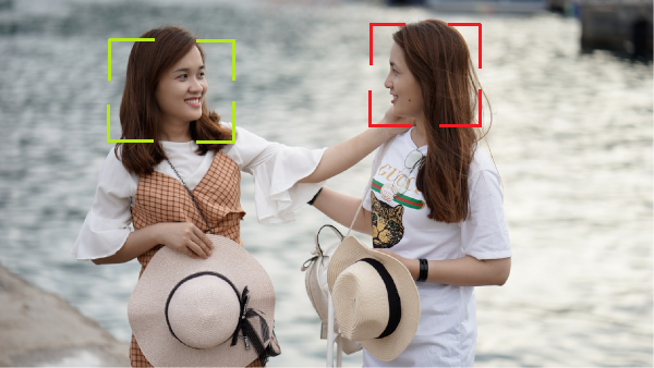
True Positive, True Negative, False Positive и False Negative
В предыдущем материале мы говорили о режимах работы биометрических платформ распознавания лиц: верификации и идентификации. Для точного результата систему предварительно обучают, а для оценки качества работы алгоритмов используют специальные метрики:
- True Positive. Положительный результат, который мы ожидали получить: лицо находилось в базе данных, и система распознала его.
- True Negative. Отрицательный результат, который мы ожидали получить: лицо не было занесено в базу данных, система не распознала его и сообщила о неизвестном посетителе.
- False Positive. Положительный результат, который оказался ошибочным: система распознала лицо чужого человека, ошибочно приняв его за другое лицо, находящееся в базе данных, и открыла доступ.
- False Negative. Отрицательный результат, который оказался ошибочным: система не распознала лицо, хотя должна была это сделать, и определила действия человека как попытку несанкционированного проникновения на объект.
Показатели False Rejection Rate и False Acceptance Rate
Для оценки эффективности работы алгоритма используют еще одни значения — процентное соотношение количества ошибок, то есть количество неверно распознанных лиц при прохождении посетителями процедуры допуска.
Учитывают два вида ошибок:
- False Rejection Rate (FRR) — ошибка первого рода, процент вероятности определения системой «своего» за «чужого» или количество отказов в допуске авторизованным лицам, имеющим право доступа. Можно сказать, это процент возникновения результата False Negative, о котором мы говорили в предыдущем абзаце. Например, показатель 1:1000 означает, что только одному человеку из 1000 авторизованных пользователей будет ошибочно отказано в доступе.
- False Acceptance Rate (FAR) — ошибка второго рода, процент вероятности принятия «чужого» за «своего» или количество ошибочных допусков системой неавторизованных лиц, то есть результата False Positive из абзаца выше. Например, показатель 1:100 000 указывает на то, что из 100 000 неавторизованных посетителей система ошибочно пропустит только одного человека.
Оба показателя важны для оценки работы алгоритма, высокий процент ошибок говорит о неэффективности системы: на контрольно-пропускном пункте для пассажиров слишком частое возникновение False Rejection приведет к образованию заторов, система помешает пройти путешественникам с законным правом доступа и создаст лишние проблемы, а при регулярном возникновении False Accept в самолет или на территорию другой страны может проникнуть злоумышленник.

Референсное изображение лица
Референсные изображения — это примеры лиц, на которых система будет обучаться, или изображения в базе данных, с которыми будет сравнивать захваченное лицо.
В обоих случаях от референсного изображения лица зависит точность распознавания. При выборе примера важны факторы:
- качество изображения лица — четкость картинки, достаточное разрешение и отсутствие дефектов,
- ракурс фотографии,
- освещение — равномерное и естественное, без резких перепадов света и тени,
- хорошо различимое лицо — без очков, головных уборов, крупных украшений и других деталей, которые могут помешать системе распознать лицо.
Важно и количество референсных изображений. Чем больше качественных примеров получит система во время обучения, тем точнее будет ее алгоритм. При использовании технологии распознавания лиц «в поле» несколько изображений одного человека, снятых с разных точек, помогут быстрее и точнее идентифицировать посетителя, кроме того, играет роль и расположение камеры — ее нужно установить под таким углом, чтобы захваченное лицо было хорошо видно.
Искусственный интеллект
Понятие «искусственный интеллект» объединяет несколько определений:
- направление науки, занимающееся разработкой компьютерных программ и систем, способных выполнять интеллектуальные функции, присущие человеку,
- искусственно созданный человеком набор алгоритмов, способных работать по аналогии с мозгом человека — принимать интеллектуальные решения, отвечать на вопросы, выполнять творческие задачи.
Искусственный интеллект создан для воспроизведения действий человеческого мозга с помощью компьютерных расчетов, он помогает машинам обрабатывать информацию и принимать решения, аналогичные человеческим. Распознавание лиц тоже относится к области искусственного интеллекта.
Искусственный интеллект используется во многих отраслях, с его помощью автоматизируют рутинные операции и процессы — сбор данных для исследований, обслуживание клиентов, сортировка товаров, круглосуточная охрана территорий и объектов.
Глубокое обучение (Deep Learning)
Для правильной работы искусственного интеллекта, в том числе технологии распознавания лиц, нужен алгоритм. Глубокое обучение — один из методов машинного обучения, основанный на принципе многослойности.
Вместо запоминания конкретного алгоритма для определенной задачи система получает комплекс данных для анализа, результаты которого учитываются при следующем анализе. Результаты каждого анализа наслаиваются, в итоге система получает набор данных, достаточных для построения собственного алгоритма для решения любой задачи.
Системы, обученные по этому принципу, не только быстро и точно выполняют свои задачи, но и могут самостоятельно принять решение в нестандартной ситуации.
По прогнозам экспертов, в ближайшие пять лет область применения технологии распознавания лиц расширится. Для посадки на самолет, снятия денег со счета, покупки машины и других действий не понадобятся документы — достаточно будет просто показать лицо.
Оценка качества Биометрических систем
Работа
биометрической системы идентификации
пользователя (БСИ) описывается техническими
и ценовыми параметрами. Качество работы
БСИ характеризуется процентом ошибок
при прохождении процедуры допуска. В
БСИ различают ошибки трех видов:
-
FRR
(False Rejection Rate)ошибка первого рода—
вероятность принять «своего» за
«чужого». Обычно в коммерческих
системах эта ошибка выбирается равной
примерно 0,01, поскольку считается, что,
разрешив несколько касаний для «своих»,
можно искусственным способом улучшить
эту ошибку. В ряде случаев (скажем, при
большом потоке, чтобы не создавать
очередей) требуется улучшение FRR до
0,001-0,0001. В системах, присутствующих на
рынке, FRR обычно находится в диапазоне
0,025-0,01. -
FAR
(False Acceptance Rate)ошибка второго рода— вероятность принять «чужого» за
«своего». В представленных на рынке
системах эта ошибка колеблется в
основном от 10-3до 10-6, хотя
есть решения и с FAR = 10-9. Чем больше
данная ошибка, тем грубее работает
система и тем вероятнее проникновение
«чужого»; поэтому в системах с
большим числом пользователей или
транзакций следует ориентироваться
на малые значения FAR.
-
EER
(Equal Error Rates)– равная вероятность
(норма) ошибок первого и второго рода.
Биометрические
технологии
основаны на биометрии, измерении
уникальных характеристик отдельно
взятого человека. Это могут быть как
уникальные признаки, полученные им с
рождения, например: ДНК, отпечатки
пальцев, радужная оболочка глаза; так
и характеристики, приобретённые со
временем или же способные меняться с
возрастом или внешним воздействием,
например: почерк, голос или походка.
Все
биометрические системы работают
практически по одинаковой схеме.
Во-первых, система запоминает образец
биометрической характеристики (это и
называется процессом записи). Во время
записи некоторые биометрические системы
могут попросить сделать несколько
образцов для того, чтобы составить
наиболее точное изображение биометрической
характеристики. Затем полученная
информация обрабатывается и
преобразовывается в математический
код. Кроме того, система может попросить
произвести ещё некоторые действия для
того, чтобы «приписать» биометрический
образец к определённому человеку.
Например, персональный идентификационный
номер (PIN) прикрепляется к определённому
образцу, либо смарт-карта, содержащая
образец, вставляется в считывающее
устройство. В таком случае, снова делается
образец биометрической характеристики
и сравнивается с представленным образцом.
Идентификация по любой биометрической
системе проходит четыре стадии:
-
Запись
– физический или поведенческий образец
запоминается системой; -
Выделение
– уникальная информация выносится из
образца и составляется биометрический
образец; -
Сравнение
– сохраненный образец сравнивается с
представленным; -
Совпадение/несовпадение
— система решает, совпадают ли
биометрические образцы, и выносит
решение.
Подавляющее
большинство людей считают, что в памяти
компьютера хранится образец отпечатка
пальца, голоса человека или картинка
радужной оболочки его глаза. Но на самом
деле в большинстве современных систем
это не так. В специальной базе данных
хранится цифровой код длиной до 1000 бит,
который ассоциируется с конкретным
человеком, имеющим право доступа. Сканер
или любое другое устройство, используемое
в системе, считывает определённый
биологический параметр человека. Далее
он обрабатывает полученное изображение
или звук, преобразовывая их в цифровой
код. Именно этот ключ и сравнивается с
содержимым специальной базы данных для
идентификации личности [19].
Преимущества
биометрической идентификации состоит
в том, что биометрическая защита дает
больший эффект по сравнению, например,
с использованием паролей, смарт-карт,
PIN-кодов, жетонов или технологии
инфраструктуры открытых ключей. Это
объясняется возможностью биометрии
идентифицировать не устройство, но
человека.
Обычные
методы защиты чреваты потерей или кражей
информации, которая становится открытой
для незаконных пользователей.
Исключительный биометрический
идентификатор, например, отпечатки
пальцев, является ключом, не подлежащим
потере [18].
Соседние файлы в папке ГОСЫ
- #
- #
- #
- #
- #
- #
- #
- #
- #
This article is about erroneous outcomes of statistical tests. For closely related concepts in binary classification and testing generally, see false positives and false negatives.
In statistical hypothesis testing, a type I error is the mistaken rejection of an actually true null hypothesis (also known as a «false positive» finding or conclusion; example: «an innocent person is convicted»), while a type II error is the failure to reject a null hypothesis that is actually false (also known as a «false negative» finding or conclusion; example: «a guilty person is not convicted»).[1] Much of statistical theory revolves around the minimization of one or both of these errors, though the complete elimination of either is a statistical impossibility if the outcome is not determined by a known, observable causal process.
By selecting a low threshold (cut-off) value and modifying the alpha (α) level, the quality of the hypothesis test can be increased.[2] The knowledge of type I errors and type II errors is widely used in medical science, biometrics and computer science.[clarification needed]
Intuitively, type I errors can be thought of as errors of commission, i.e. the researcher unluckily concludes that something is the fact. For instance, consider a study where researchers compare a drug with a placebo. If the patients who are given the drug get better than the patients given the placebo by chance, it may appear that the drug is effective, but in fact the conclusion is incorrect.
In reverse, type II errors are errors of omission. In the example above, if the patients who got the drug did not get better at a higher rate than the ones who got the placebo, but this was a random fluke, that would be a type II error. The consequence of a type II error depends on the size and direction of the missed determination and the circumstances. An expensive cure for one in a million patients may be inconsequential even if it truly is a cure.
Definition[edit]
Statistical background[edit]
In statistical test theory, the notion of a statistical error is an integral part of hypothesis testing. The test goes about choosing about two competing propositions called null hypothesis, denoted by H0 and alternative hypothesis, denoted by H1. This is conceptually similar to the judgement in a court trial. The null hypothesis corresponds to the position of the defendant: just as he is presumed to be innocent until proven guilty, so is the null hypothesis presumed to be true until the data provide convincing evidence against it. The alternative hypothesis corresponds to the position against the defendant. Specifically, the null hypothesis also involves the absence of a difference or the absence of an association. Thus, the null hypothesis can never be that there is a difference or an association.
If the result of the test corresponds with reality, then a correct decision has been made. However, if the result of the test does not correspond with reality, then an error has occurred. There are two situations in which the decision is wrong. The null hypothesis may be true, whereas we reject H0. On the other hand, the alternative hypothesis H1 may be true, whereas we do not reject H0. Two types of error are distinguished: type I error and type II error.[3]
Type I error[edit]
The first kind of error is the mistaken rejection of a null hypothesis as the result of a test procedure. This kind of error is called a type I error (false positive) and is sometimes called an error of the first kind. In terms of the courtroom example, a type I error corresponds to convicting an innocent defendant.
Type II error[edit]
The second kind of error is the mistaken failure to reject the null hypothesis as the result of a test procedure. This sort of error is called a type II error (false negative) and is also referred to as an error of the second kind. In terms of the courtroom example, a type II error corresponds to acquitting a criminal.[4]
Crossover error rate[edit]
The crossover error rate (CER) is the point at which type I errors and type II errors are equal. A system with a lower CER value provides more accuracy than a system with a higher CER value.
False positive and false negative[edit]
In terms of false positives and false negatives, a positive result corresponds to rejecting the null hypothesis, while a negative result corresponds to failing to reject the null hypothesis; «false» means the conclusion drawn is incorrect. Thus, a type I error is equivalent to a false positive, and a type II error is equivalent to a false negative.
Table of error types[edit]
Tabularised relations between truth/falseness of the null hypothesis and outcomes of the test:[5]
| Table of error types | Null hypothesis (H0) is |
||
|---|---|---|---|
| True | False | ||
| Decision about null hypothesis (H0) |
Don’t reject |
Correct inference (true negative) (probability = 1−α) |
Type II error (false negative) (probability = β) |
| Reject | Type I error (false positive) (probability = α) |
Correct inference (true positive) (probability = 1−β) |
Error rate[edit]

The results obtained from negative sample (left curve) overlap with the results obtained from positive samples (right curve). By moving the result cutoff value (vertical bar), the rate of false positives (FP) can be decreased, at the cost of raising the number of false negatives (FN), or vice versa (TP = True Positives, TPR = True Positive Rate, FPR = False Positive Rate, TN = True Negatives).
A perfect test would have zero false positives and zero false negatives. However, statistical methods are probabilistic, and it cannot be known for certain whether statistical conclusions are correct. Whenever there is uncertainty, there is the possibility of making an error. Considering this nature of statistics science, all statistical hypothesis tests have a probability of making type I and type II errors.[6]
- The type I error rate is the probability of rejecting the null hypothesis given that it is true. The test is designed to keep the type I error rate below a prespecified bound called the significance level, usually denoted by the Greek letter α (alpha) and is also called the alpha level. Usually, the significance level is set to 0.05 (5%), implying that it is acceptable to have a 5% probability of incorrectly rejecting the true null hypothesis.[7]
- The rate of the type II error is denoted by the Greek letter β (beta) and related to the power of a test, which equals 1−β.[8]
These two types of error rates are traded off against each other: for any given sample set, the effort to reduce one type of error generally results in increasing the other type of error.[9]
The quality of hypothesis test[edit]
The same idea can be expressed in terms of the rate of correct results and therefore used to minimize error rates and improve the quality of hypothesis test. To reduce the probability of committing a type I error, making the alpha value more stringent is quite simple and efficient. To decrease the probability of committing a type II error, which is closely associated with analyses’ power, either increasing the test’s sample size or relaxing the alpha level could increase the analyses’ power.[10] A test statistic is robust if the type I error rate is controlled.
Varying different threshold (cut-off) value could also be used to make the test either more specific or more sensitive, which in turn elevates the test quality. For example, imagine a medical test, in which an experimenter might measure the concentration of a certain protein in the blood sample. The experimenter could adjust the threshold (black vertical line in the figure) and people would be diagnosed as having diseases if any number is detected above this certain threshold. According to the image, changing the threshold would result in changes in false positives and false negatives, corresponding to movement on the curve.[11]
Example[edit]
Since in a real experiment it is impossible to avoid all type I and type II errors, it is important to consider the amount of risk one is willing to take to falsely reject H0 or accept H0. The solution to this question would be to report the p-value or significance level α of the statistic. For example, if the p-value of a test statistic result is estimated at 0.0596, then there is a probability of 5.96% that we falsely reject H0. Or, if we say, the statistic is performed at level α, like 0.05, then we allow to falsely reject H0 at 5%. A significance level α of 0.05 is relatively common, but there is no general rule that fits all scenarios.
Vehicle speed measuring[edit]
The speed limit of a freeway in the United States is 120 kilometers per hour. A device is set to measure the speed of passing vehicles. Suppose that the device will conduct three measurements of the speed of a passing vehicle, recording as a random sample X1, X2, X3. The traffic police will or will not fine the drivers depending on the average speed 

In addition, we suppose that the measurements X1, X2, X3 are modeled as normal distribution N(μ,4). Then, T should follow N(μ,4/3) and the parameter μ represents the true speed of passing vehicle. In this experiment, the null hypothesis H0 and the alternative hypothesis H1 should be
H0: μ=120 against H1: μ1>120.
If we perform the statistic level at α=0.05, then a critical value c should be calculated to solve
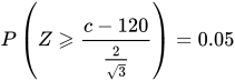
According to change-of-units rule for the normal distribution. Referring to Z-table, we can get
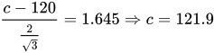
Here, the critical region. That is to say, if the recorded speed of a vehicle is greater than critical value 121.9, the driver will be fined. However, there are still 5% of the drivers are falsely fined since the recorded average speed is greater than 121.9 but the true speed does not pass 120, which we say, a type I error.
The type II error corresponds to the case that the true speed of a vehicle is over 120 kilometers per hour but the driver is not fined. For example, if the true speed of a vehicle μ=125, the probability that the driver is not fined can be calculated as

which means, if the true speed of a vehicle is 125, the driver has the probability of 0.36% to avoid the fine when the statistic is performed at level 125 since the recorded average speed is lower than 121.9. If the true speed is closer to 121.9 than 125, then the probability of avoiding the fine will also be higher.
The tradeoffs between type I error and type II error should also be considered. That is, in this case, if the traffic police do not want to falsely fine innocent drivers, the level α can be set to a smaller value, like 0.01. However, if that is the case, more drivers whose true speed is over 120 kilometers per hour, like 125, would be more likely to avoid the fine.
Etymology[edit]
In 1928, Jerzy Neyman (1894–1981) and Egon Pearson (1895–1980), both eminent statisticians, discussed the problems associated with «deciding whether or not a particular sample may be judged as likely to have been randomly drawn from a certain population»:[12] and, as Florence Nightingale David remarked, «it is necessary to remember the adjective ‘random’ [in the term ‘random sample’] should apply to the method of drawing the sample and not to the sample itself».[13]
They identified «two sources of error», namely:
- (a) the error of rejecting a hypothesis that should have not been rejected, and
- (b) the error of failing to reject a hypothesis that should have been rejected.
In 1930, they elaborated on these two sources of error, remarking that:
…in testing hypotheses two considerations must be kept in view, we must be able to reduce the chance of rejecting a true hypothesis to as low a value as desired; the test must be so devised that it will reject the hypothesis tested when it is likely to be false.
In 1933, they observed that these «problems are rarely presented in such a form that we can discriminate with certainty between the true and false hypothesis» . They also noted that, in deciding whether to fail to reject, or reject a particular hypothesis amongst a «set of alternative hypotheses», H1, H2…, it was easy to make an error:
…[and] these errors will be of two kinds:
- (I) we reject H0 [i.e., the hypothesis to be tested] when it is true,[14]
- (II) we fail to reject H0 when some alternative hypothesis HA or H1 is true. (There are various notations for the alternative).
In all of the papers co-written by Neyman and Pearson the expression H0 always signifies «the hypothesis to be tested».
In the same paper they call these two sources of error, errors of type I and errors of type II respectively.[15]
[edit]
Null hypothesis[edit]
It is standard practice for statisticians to conduct tests in order to determine whether or not a «speculative hypothesis» concerning the observed phenomena of the world (or its inhabitants) can be supported. The results of such testing determine whether a particular set of results agrees reasonably (or does not agree) with the speculated hypothesis.
On the basis that it is always assumed, by statistical convention, that the speculated hypothesis is wrong, and the so-called «null hypothesis» that the observed phenomena simply occur by chance (and that, as a consequence, the speculated agent has no effect) – the test will determine whether this hypothesis is right or wrong. This is why the hypothesis under test is often called the null hypothesis (most likely, coined by Fisher (1935, p. 19)), because it is this hypothesis that is to be either nullified or not nullified by the test. When the null hypothesis is nullified, it is possible to conclude that data support the «alternative hypothesis» (which is the original speculated one).
The consistent application by statisticians of Neyman and Pearson’s convention of representing «the hypothesis to be tested» (or «the hypothesis to be nullified») with the expression H0 has led to circumstances where many understand the term «the null hypothesis» as meaning «the nil hypothesis» – a statement that the results in question have arisen through chance. This is not necessarily the case – the key restriction, as per Fisher (1966), is that «the null hypothesis must be exact, that is free from vagueness and ambiguity, because it must supply the basis of the ‘problem of distribution,’ of which the test of significance is the solution.»[16] As a consequence of this, in experimental science the null hypothesis is generally a statement that a particular treatment has no effect; in observational science, it is that there is no difference between the value of a particular measured variable, and that of an experimental prediction.[citation needed]
Statistical significance[edit]
If the probability of obtaining a result as extreme as the one obtained, supposing that the null hypothesis were true, is lower than a pre-specified cut-off probability (for example, 5%), then the result is said to be statistically significant and the null hypothesis is rejected.
British statistician Sir Ronald Aylmer Fisher (1890–1962) stressed that the «null hypothesis»:
… is never proved or established, but is possibly disproved, in the course of experimentation. Every experiment may be said to exist only in order to give the facts a chance of disproving the null hypothesis.
— Fisher, 1935, p.19
Application domains[edit]
Medicine[edit]
In the practice of medicine, the differences between the applications of screening and testing are considerable.
Medical screening[edit]
Screening involves relatively cheap tests that are given to large populations, none of whom manifest any clinical indication of disease (e.g., Pap smears).
Testing involves far more expensive, often invasive, procedures that are given only to those who manifest some clinical indication of disease, and are most often applied to confirm a suspected diagnosis.
For example, most states in the USA require newborns to be screened for phenylketonuria and hypothyroidism, among other congenital disorders.
Hypothesis: «The newborns have phenylketonuria and hypothyroidism»
Null Hypothesis (H0): «The newborns do not have phenylketonuria and hypothyroidism»,
Type I error (false positive): The true fact is that the newborns do not have phenylketonuria and hypothyroidism but we consider they have the disorders according to the data.
Type II error (false negative): The true fact is that the newborns have phenylketonuria and hypothyroidism but we consider they do not have the disorders according to the data.
Although they display a high rate of false positives, the screening tests are considered valuable because they greatly increase the likelihood of detecting these disorders at a far earlier stage.
The simple blood tests used to screen possible blood donors for HIV and hepatitis have a significant rate of false positives; however, physicians use much more expensive and far more precise tests to determine whether a person is actually infected with either of these viruses.
Perhaps the most widely discussed false positives in medical screening come from the breast cancer screening procedure mammography. The US rate of false positive mammograms is up to 15%, the highest in world. One consequence of the high false positive rate in the US is that, in any 10-year period, half of the American women screened receive a false positive mammogram. False positive mammograms are costly, with over $100 million spent annually in the U.S. on follow-up testing and treatment. They also cause women unneeded anxiety. As a result of the high false positive rate in the US, as many as 90–95% of women who get a positive mammogram do not have the condition. The lowest rate in the world is in the Netherlands, 1%. The lowest rates are generally in Northern Europe where mammography films are read twice and a high threshold for additional testing is set (the high threshold decreases the power of the test).
The ideal population screening test would be cheap, easy to administer, and produce zero false-negatives, if possible. Such tests usually produce more false-positives, which can subsequently be sorted out by more sophisticated (and expensive) testing.
Medical testing[edit]
False negatives and false positives are significant issues in medical testing.
Hypothesis: «The patients have the specific disease».
Null hypothesis (H0): «The patients do not have the specific disease».
Type I error (false positive): «The true fact is that the patients do not have a specific disease but the physicians judges the patients was ill according to the test reports».
False positives can also produce serious and counter-intuitive problems when the condition being searched for is rare, as in screening. If a test has a false positive rate of one in ten thousand, but only one in a million samples (or people) is a true positive, most of the positives detected by that test will be false. The probability that an observed positive result is a false positive may be calculated using Bayes’ theorem.
Type II error (false negative): «The true fact is that the disease is actually present but the test reports provide a falsely reassuring message to patients and physicians that the disease is absent».
False negatives produce serious and counter-intuitive problems, especially when the condition being searched for is common. If a test with a false negative rate of only 10% is used to test a population with a true occurrence rate of 70%, many of the negatives detected by the test will be false.
This sometimes leads to inappropriate or inadequate treatment of both the patient and their disease. A common example is relying on cardiac stress tests to detect coronary atherosclerosis, even though cardiac stress tests are known to only detect limitations of coronary artery blood flow due to advanced stenosis.
Biometrics[edit]
Biometric matching, such as for fingerprint recognition, facial recognition or iris recognition, is susceptible to type I and type II errors.
Hypothesis: «The input does not identify someone in the searched list of people»
Null hypothesis: «The input does identify someone in the searched list of people»
Type I error (false reject rate): «The true fact is that the person is someone in the searched list but the system concludes that the person is not according to the data».
Type II error (false match rate): «The true fact is that the person is not someone in the searched list but the system concludes that the person is someone whom we are looking for according to the data».
The probability of type I errors is called the «false reject rate» (FRR) or false non-match rate (FNMR), while the probability of type II errors is called the «false accept rate» (FAR) or false match rate (FMR).
If the system is designed to rarely match suspects then the probability of type II errors can be called the «false alarm rate». On the other hand, if the system is used for validation (and acceptance is the norm) then the FAR is a measure of system security, while the FRR measures user inconvenience level.
Security screening[edit]
False positives are routinely found every day in airport security screening, which are ultimately visual inspection systems. The installed security alarms are intended to prevent weapons being brought onto aircraft; yet they are often set to such high sensitivity that they alarm many times a day for minor items, such as keys, belt buckles, loose change, mobile phones, and tacks in shoes.
Here, the null hypothesis is that the item is not a weapon, while the alternative hypothesis is that the item is a weapon.
A type I error (false positive): «The true fact is that the item is not a weapon but the system still alarms».
Type II error (false negative) «The true fact is that the item is a weapon but the system keeps silent at this time».
The ratio of false positives (identifying an innocent traveler as a terrorist) to true positives (detecting a would-be terrorist) is, therefore, very high; and because almost every alarm is a false positive, the positive predictive value of these screening tests is very low.
The relative cost of false results determines the likelihood that test creators allow these events to occur. As the cost of a false negative in this scenario is extremely high (not detecting a bomb being brought onto a plane could result in hundreds of deaths) whilst the cost of a false positive is relatively low (a reasonably simple further inspection) the most appropriate test is one with a low statistical specificity but high statistical sensitivity (one that allows a high rate of false positives in return for minimal false negatives).
Computers[edit]
The notions of false positives and false negatives have a wide currency in the realm of computers and computer applications, including computer security, spam filtering, Malware, Optical character recognition and many others.
For example, in the case of spam filtering the hypothesis here is that the message is a spam.
Thus, null hypothesis: «The message is not a spam».
Type I error (false positive): «Spam filtering or spam blocking techniques wrongly classify a legitimate email message as spam and, as a result, interferes with its delivery».
While most anti-spam tactics can block or filter a high percentage of unwanted emails, doing so without creating significant false-positive results is a much more demanding task.
Type II error (false negative): «Spam email is not detected as spam, but is classified as non-spam». A low number of false negatives is an indicator of the efficiency of spam filtering.
See also[edit]
- Binary classification
- Detection theory
- Egon Pearson
- Ethics in mathematics
- False positive paradox
- False discovery rate
- Family-wise error rate
- Information retrieval performance measures
- Neyman–Pearson lemma
- Null hypothesis
- Probability of a hypothesis for Bayesian inference
- Precision and recall
- Prosecutor’s fallacy
- Prozone phenomenon
- Receiver operating characteristic
- Sensitivity and specificity
- Statisticians’ and engineers’ cross-reference of statistical terms
- Testing hypotheses suggested by the data
- Type III error
References[edit]
- ^ «Type I Error and Type II Error». explorable.com. Retrieved 14 December 2019.
- ^ Chow, Y. W.; Pietranico, R.; Mukerji, A. (27 October 1975). «Studies of oxygen binding energy to hemoglobin molecule». Biochemical and Biophysical Research Communications. 66 (4): 1424–1431. doi:10.1016/0006-291x(75)90518-5. ISSN 0006-291X. PMID 6.
- ^ A modern introduction to probability and statistics : understanding why and how. Dekking, Michel, 1946-. London: Springer. 2005. ISBN 978-1-85233-896-1. OCLC 262680588.
{{cite book}}: CS1 maint: others (link) - ^ A modern introduction to probability and statistics : understanding why and how. Dekking, Michel, 1946-. London: Springer. 2005. ISBN 978-1-85233-896-1. OCLC 262680588.
{{cite book}}: CS1 maint: others (link) - ^ Sheskin, David (2004). Handbook of Parametric and Nonparametric Statistical Procedures. CRC Press. p. 54. ISBN 1584884401.
- ^ Smith, R. J.; Bryant, R. G. (27 October 1975). «Metal substitutions incarbonic anhydrase: a halide ion probe study». Biochemical and Biophysical Research Communications. 66 (4): 1281–1286. doi:10.1016/0006-291x(75)90498-2. ISSN 0006-291X. PMC 9650581. PMID 3.
- ^ Lindenmayer, David. (2005). Practical conservation biology. Burgman, Mark A. Collingwood, Vic.: CSIRO Pub. ISBN 0-643-09310-9. OCLC 65216357.
- ^ Chow, Y. W.; Pietranico, R.; Mukerji, A. (27 October 1975). «Studies of oxygen binding energy to hemoglobin molecule». Biochemical and Biophysical Research Communications. 66 (4): 1424–1431. doi:10.1016/0006-291x(75)90518-5. ISSN 0006-291X. PMID 6.
- ^ Smith, R. J.; Bryant, R. G. (27 October 1975). «Metal substitutions incarbonic anhydrase: a halide ion probe study». Biochemical and Biophysical Research Communications. 66 (4): 1281–1286. doi:10.1016/0006-291x(75)90498-2. ISSN 0006-291X. PMC 9650581. PMID 3.
- ^ Smith, R. J.; Bryant, R. G. (27 October 1975). «Metal substitutions incarbonic anhydrase: a halide ion probe study». Biochemical and Biophysical Research Communications. 66 (4): 1281–1286. doi:10.1016/0006-291x(75)90498-2. ISSN 0006-291X. PMC 9650581. PMID 3.
- ^ Moroi, K.; Sato, T. (15 August 1975). «Comparison between procaine and isocarboxazid metabolism in vitro by a liver microsomal amidase-esterase». Biochemical Pharmacology. 24 (16): 1517–1521. doi:10.1016/0006-2952(75)90029-5. ISSN 1873-2968. PMID 8.
- ^ NEYMAN, J.; PEARSON, E. S. (1928). «On the Use and Interpretation of Certain Test Criteria for Purposes of Statistical Inference Part I». Biometrika. 20A (1–2): 175–240. doi:10.1093/biomet/20a.1-2.175. ISSN 0006-3444.
- ^ C.I.K.F. (July 1951). «Probability Theory for Statistical Methods. By F. N. David. [Pp. ix + 230. Cambridge University Press. 1949. Price 155.]». Journal of the Staple Inn Actuarial Society. 10 (3): 243–244. doi:10.1017/s0020269x00004564. ISSN 0020-269X.
- ^ Note that the subscript in the expression H0 is a zero (indicating null), and is not an «O» (indicating original).
- ^ Neyman, J.; Pearson, E. S. (30 October 1933). «The testing of statistical hypotheses in relation to probabilities a priori». Mathematical Proceedings of the Cambridge Philosophical Society. 29 (4): 492–510. Bibcode:1933PCPS…29..492N. doi:10.1017/s030500410001152x. ISSN 0305-0041. S2CID 119855116.
- ^ Fisher, R.A. (1966). The design of experiments. 8th edition. Hafner:Edinburgh.
Bibliography[edit]
- Betz, M.A. & Gabriel, K.R., «Type IV Errors and Analysis of Simple Effects», Journal of Educational Statistics, Vol.3, No.2, (Summer 1978), pp. 121–144.
- David, F.N., «A Power Function for Tests of Randomness in a Sequence of Alternatives», Biometrika, Vol.34, Nos.3/4, (December 1947), pp. 335–339.
- Fisher, R.A., The Design of Experiments, Oliver & Boyd (Edinburgh), 1935.
- Gambrill, W., «False Positives on Newborns’ Disease Tests Worry Parents», Health Day, (5 June 2006). [1] Archived 17 May 2018 at the Wayback Machine
- Kaiser, H.F., «Directional Statistical Decisions», Psychological Review, Vol.67, No.3, (May 1960), pp. 160–167.
- Kimball, A.W., «Errors of the Third Kind in Statistical Consulting», Journal of the American Statistical Association, Vol.52, No.278, (June 1957), pp. 133–142.
- Lubin, A., «The Interpretation of Significant Interaction», Educational and Psychological Measurement, Vol.21, No.4, (Winter 1961), pp. 807–817.
- Marascuilo, L.A. & Levin, J.R., «Appropriate Post Hoc Comparisons for Interaction and nested Hypotheses in Analysis of Variance Designs: The Elimination of Type-IV Errors», American Educational Research Journal, Vol.7., No.3, (May 1970), pp. 397–421.
- Mitroff, I.I. & Featheringham, T.R., «On Systemic Problem Solving and the Error of the Third Kind», Behavioral Science, Vol.19, No.6, (November 1974), pp. 383–393.
- Mosteller, F., «A k-Sample Slippage Test for an Extreme Population», The Annals of Mathematical Statistics, Vol.19, No.1, (March 1948), pp. 58–65.
- Moulton, R.T., «Network Security», Datamation, Vol.29, No.7, (July 1983), pp. 121–127.
- Raiffa, H., Decision Analysis: Introductory Lectures on Choices Under Uncertainty, Addison–Wesley, (Reading), 1968.
External links[edit]
- Bias and Confounding – presentation by Nigel Paneth, Graduate School of Public Health, University of Pittsburgh
This article is about erroneous outcomes of statistical tests. For closely related concepts in binary classification and testing generally, see false positives and false negatives.
In statistical hypothesis testing, a type I error is the mistaken rejection of an actually true null hypothesis (also known as a «false positive» finding or conclusion; example: «an innocent person is convicted»), while a type II error is the failure to reject a null hypothesis that is actually false (also known as a «false negative» finding or conclusion; example: «a guilty person is not convicted»).[1] Much of statistical theory revolves around the minimization of one or both of these errors, though the complete elimination of either is a statistical impossibility if the outcome is not determined by a known, observable causal process.
By selecting a low threshold (cut-off) value and modifying the alpha (α) level, the quality of the hypothesis test can be increased.[2] The knowledge of type I errors and type II errors is widely used in medical science, biometrics and computer science.[clarification needed]
Intuitively, type I errors can be thought of as errors of commission, i.e. the researcher unluckily concludes that something is the fact. For instance, consider a study where researchers compare a drug with a placebo. If the patients who are given the drug get better than the patients given the placebo by chance, it may appear that the drug is effective, but in fact the conclusion is incorrect.
In reverse, type II errors are errors of omission. In the example above, if the patients who got the drug did not get better at a higher rate than the ones who got the placebo, but this was a random fluke, that would be a type II error. The consequence of a type II error depends on the size and direction of the missed determination and the circumstances. An expensive cure for one in a million patients may be inconsequential even if it truly is a cure.
Definition[edit]
Statistical background[edit]
In statistical test theory, the notion of a statistical error is an integral part of hypothesis testing. The test goes about choosing about two competing propositions called null hypothesis, denoted by H0 and alternative hypothesis, denoted by H1. This is conceptually similar to the judgement in a court trial. The null hypothesis corresponds to the position of the defendant: just as he is presumed to be innocent until proven guilty, so is the null hypothesis presumed to be true until the data provide convincing evidence against it. The alternative hypothesis corresponds to the position against the defendant. Specifically, the null hypothesis also involves the absence of a difference or the absence of an association. Thus, the null hypothesis can never be that there is a difference or an association.
If the result of the test corresponds with reality, then a correct decision has been made. However, if the result of the test does not correspond with reality, then an error has occurred. There are two situations in which the decision is wrong. The null hypothesis may be true, whereas we reject H0. On the other hand, the alternative hypothesis H1 may be true, whereas we do not reject H0. Two types of error are distinguished: type I error and type II error.[3]
Type I error[edit]
The first kind of error is the mistaken rejection of a null hypothesis as the result of a test procedure. This kind of error is called a type I error (false positive) and is sometimes called an error of the first kind. In terms of the courtroom example, a type I error corresponds to convicting an innocent defendant.
Type II error[edit]
The second kind of error is the mistaken failure to reject the null hypothesis as the result of a test procedure. This sort of error is called a type II error (false negative) and is also referred to as an error of the second kind. In terms of the courtroom example, a type II error corresponds to acquitting a criminal.[4]
Crossover error rate[edit]
The crossover error rate (CER) is the point at which type I errors and type II errors are equal. A system with a lower CER value provides more accuracy than a system with a higher CER value.
False positive and false negative[edit]
In terms of false positives and false negatives, a positive result corresponds to rejecting the null hypothesis, while a negative result corresponds to failing to reject the null hypothesis; «false» means the conclusion drawn is incorrect. Thus, a type I error is equivalent to a false positive, and a type II error is equivalent to a false negative.
Table of error types[edit]
Tabularised relations between truth/falseness of the null hypothesis and outcomes of the test:[5]
| Table of error types | Null hypothesis (H0) is |
||
|---|---|---|---|
| True | False | ||
| Decision about null hypothesis (H0) |
Don’t reject |
Correct inference (true negative) (probability = 1−α) |
Type II error (false negative) (probability = β) |
| Reject | Type I error (false positive) (probability = α) |
Correct inference (true positive) (probability = 1−β) |
Error rate[edit]
The results obtained from negative sample (left curve) overlap with the results obtained from positive samples (right curve). By moving the result cutoff value (vertical bar), the rate of false positives (FP) can be decreased, at the cost of raising the number of false negatives (FN), or vice versa (TP = True Positives, TPR = True Positive Rate, FPR = False Positive Rate, TN = True Negatives).
A perfect test would have zero false positives and zero false negatives. However, statistical methods are probabilistic, and it cannot be known for certain whether statistical conclusions are correct. Whenever there is uncertainty, there is the possibility of making an error. Considering this nature of statistics science, all statistical hypothesis tests have a probability of making type I and type II errors.[6]
- The type I error rate is the probability of rejecting the null hypothesis given that it is true. The test is designed to keep the type I error rate below a prespecified bound called the significance level, usually denoted by the Greek letter α (alpha) and is also called the alpha level. Usually, the significance level is set to 0.05 (5%), implying that it is acceptable to have a 5% probability of incorrectly rejecting the true null hypothesis.[7]
- The rate of the type II error is denoted by the Greek letter β (beta) and related to the power of a test, which equals 1−β.[8]
These two types of error rates are traded off against each other: for any given sample set, the effort to reduce one type of error generally results in increasing the other type of error.[9]
The quality of hypothesis test[edit]
The same idea can be expressed in terms of the rate of correct results and therefore used to minimize error rates and improve the quality of hypothesis test. To reduce the probability of committing a type I error, making the alpha value more stringent is quite simple and efficient. To decrease the probability of committing a type II error, which is closely associated with analyses’ power, either increasing the test’s sample size or relaxing the alpha level could increase the analyses’ power.[10] A test statistic is robust if the type I error rate is controlled.
Varying different threshold (cut-off) value could also be used to make the test either more specific or more sensitive, which in turn elevates the test quality. For example, imagine a medical test, in which an experimenter might measure the concentration of a certain protein in the blood sample. The experimenter could adjust the threshold (black vertical line in the figure) and people would be diagnosed as having diseases if any number is detected above this certain threshold. According to the image, changing the threshold would result in changes in false positives and false negatives, corresponding to movement on the curve.[11]
Example[edit]
Since in a real experiment it is impossible to avoid all type I and type II errors, it is important to consider the amount of risk one is willing to take to falsely reject H0 or accept H0. The solution to this question would be to report the p-value or significance level α of the statistic. For example, if the p-value of a test statistic result is estimated at 0.0596, then there is a probability of 5.96% that we falsely reject H0. Or, if we say, the statistic is performed at level α, like 0.05, then we allow to falsely reject H0 at 5%. A significance level α of 0.05 is relatively common, but there is no general rule that fits all scenarios.
Vehicle speed measuring[edit]
The speed limit of a freeway in the United States is 120 kilometers per hour. A device is set to measure the speed of passing vehicles. Suppose that the device will conduct three measurements of the speed of a passing vehicle, recording as a random sample X1, X2, X3. The traffic police will or will not fine the drivers depending on the average speed
In addition, we suppose that the measurements X1, X2, X3 are modeled as normal distribution N(μ,4). Then, T should follow N(μ,4/3) and the parameter μ represents the true speed of passing vehicle. In this experiment, the null hypothesis H0 and the alternative hypothesis H1 should be
H0: μ=120 against H1: μ1>120.
If we perform the statistic level at α=0.05, then a critical value c should be calculated to solve
According to change-of-units rule for the normal distribution. Referring to Z-table, we can get
Here, the critical region. That is to say, if the recorded speed of a vehicle is greater than critical value 121.9, the driver will be fined. However, there are still 5% of the drivers are falsely fined since the recorded average speed is greater than 121.9 but the true speed does not pass 120, which we say, a type I error.
The type II error corresponds to the case that the true speed of a vehicle is over 120 kilometers per hour but the driver is not fined. For example, if the true speed of a vehicle μ=125, the probability that the driver is not fined can be calculated as
which means, if the true speed of a vehicle is 125, the driver has the probability of 0.36% to avoid the fine when the statistic is performed at level 125 since the recorded average speed is lower than 121.9. If the true speed is closer to 121.9 than 125, then the probability of avoiding the fine will also be higher.
The tradeoffs between type I error and type II error should also be considered. That is, in this case, if the traffic police do not want to falsely fine innocent drivers, the level α can be set to a smaller value, like 0.01. However, if that is the case, more drivers whose true speed is over 120 kilometers per hour, like 125, would be more likely to avoid the fine.
Etymology[edit]
In 1928, Jerzy Neyman (1894–1981) and Egon Pearson (1895–1980), both eminent statisticians, discussed the problems associated with «deciding whether or not a particular sample may be judged as likely to have been randomly drawn from a certain population»:[12] and, as Florence Nightingale David remarked, «it is necessary to remember the adjective ‘random’ [in the term ‘random sample’] should apply to the method of drawing the sample and not to the sample itself».[13]
They identified «two sources of error», namely:
- (a) the error of rejecting a hypothesis that should have not been rejected, and
- (b) the error of failing to reject a hypothesis that should have been rejected.
In 1930, they elaborated on these two sources of error, remarking that:
…in testing hypotheses two considerations must be kept in view, we must be able to reduce the chance of rejecting a true hypothesis to as low a value as desired; the test must be so devised that it will reject the hypothesis tested when it is likely to be false.
In 1933, they observed that these «problems are rarely presented in such a form that we can discriminate with certainty between the true and false hypothesis» . They also noted that, in deciding whether to fail to reject, or reject a particular hypothesis amongst a «set of alternative hypotheses», H1, H2…, it was easy to make an error:
…[and] these errors will be of two kinds:
- (I) we reject H0 [i.e., the hypothesis to be tested] when it is true,[14]
- (II) we fail to reject H0 when some alternative hypothesis HA or H1 is true. (There are various notations for the alternative).
In all of the papers co-written by Neyman and Pearson the expression H0 always signifies «the hypothesis to be tested».
In the same paper they call these two sources of error, errors of type I and errors of type II respectively.[15]
[edit]
Null hypothesis[edit]
It is standard practice for statisticians to conduct tests in order to determine whether or not a «speculative hypothesis» concerning the observed phenomena of the world (or its inhabitants) can be supported. The results of such testing determine whether a particular set of results agrees reasonably (or does not agree) with the speculated hypothesis.
On the basis that it is always assumed, by statistical convention, that the speculated hypothesis is wrong, and the so-called «null hypothesis» that the observed phenomena simply occur by chance (and that, as a consequence, the speculated agent has no effect) – the test will determine whether this hypothesis is right or wrong. This is why the hypothesis under test is often called the null hypothesis (most likely, coined by Fisher (1935, p. 19)), because it is this hypothesis that is to be either nullified or not nullified by the test. When the null hypothesis is nullified, it is possible to conclude that data support the «alternative hypothesis» (which is the original speculated one).
The consistent application by statisticians of Neyman and Pearson’s convention of representing «the hypothesis to be tested» (or «the hypothesis to be nullified») with the expression H0 has led to circumstances where many understand the term «the null hypothesis» as meaning «the nil hypothesis» – a statement that the results in question have arisen through chance. This is not necessarily the case – the key restriction, as per Fisher (1966), is that «the null hypothesis must be exact, that is free from vagueness and ambiguity, because it must supply the basis of the ‘problem of distribution,’ of which the test of significance is the solution.»[16] As a consequence of this, in experimental science the null hypothesis is generally a statement that a particular treatment has no effect; in observational science, it is that there is no difference between the value of a particular measured variable, and that of an experimental prediction.[citation needed]
Statistical significance[edit]
If the probability of obtaining a result as extreme as the one obtained, supposing that the null hypothesis were true, is lower than a pre-specified cut-off probability (for example, 5%), then the result is said to be statistically significant and the null hypothesis is rejected.
British statistician Sir Ronald Aylmer Fisher (1890–1962) stressed that the «null hypothesis»:
… is never proved or established, but is possibly disproved, in the course of experimentation. Every experiment may be said to exist only in order to give the facts a chance of disproving the null hypothesis.
— Fisher, 1935, p.19
Application domains[edit]
Medicine[edit]
In the practice of medicine, the differences between the applications of screening and testing are considerable.
Medical screening[edit]
Screening involves relatively cheap tests that are given to large populations, none of whom manifest any clinical indication of disease (e.g., Pap smears).
Testing involves far more expensive, often invasive, procedures that are given only to those who manifest some clinical indication of disease, and are most often applied to confirm a suspected diagnosis.
For example, most states in the USA require newborns to be screened for phenylketonuria and hypothyroidism, among other congenital disorders.
Hypothesis: «The newborns have phenylketonuria and hypothyroidism»
Null Hypothesis (H0): «The newborns do not have phenylketonuria and hypothyroidism»,
Type I error (false positive): The true fact is that the newborns do not have phenylketonuria and hypothyroidism but we consider they have the disorders according to the data.
Type II error (false negative): The true fact is that the newborns have phenylketonuria and hypothyroidism but we consider they do not have the disorders according to the data.
Although they display a high rate of false positives, the screening tests are considered valuable because they greatly increase the likelihood of detecting these disorders at a far earlier stage.
The simple blood tests used to screen possible blood donors for HIV and hepatitis have a significant rate of false positives; however, physicians use much more expensive and far more precise tests to determine whether a person is actually infected with either of these viruses.
Perhaps the most widely discussed false positives in medical screening come from the breast cancer screening procedure mammography. The US rate of false positive mammograms is up to 15%, the highest in world. One consequence of the high false positive rate in the US is that, in any 10-year period, half of the American women screened receive a false positive mammogram. False positive mammograms are costly, with over $100 million spent annually in the U.S. on follow-up testing and treatment. They also cause women unneeded anxiety. As a result of the high false positive rate in the US, as many as 90–95% of women who get a positive mammogram do not have the condition. The lowest rate in the world is in the Netherlands, 1%. The lowest rates are generally in Northern Europe where mammography films are read twice and a high threshold for additional testing is set (the high threshold decreases the power of the test).
The ideal population screening test would be cheap, easy to administer, and produce zero false-negatives, if possible. Such tests usually produce more false-positives, which can subsequently be sorted out by more sophisticated (and expensive) testing.
Medical testing[edit]
False negatives and false positives are significant issues in medical testing.
Hypothesis: «The patients have the specific disease».
Null hypothesis (H0): «The patients do not have the specific disease».
Type I error (false positive): «The true fact is that the patients do not have a specific disease but the physicians judges the patients was ill according to the test reports».
False positives can also produce serious and counter-intuitive problems when the condition being searched for is rare, as in screening. If a test has a false positive rate of one in ten thousand, but only one in a million samples (or people) is a true positive, most of the positives detected by that test will be false. The probability that an observed positive result is a false positive may be calculated using Bayes’ theorem.
Type II error (false negative): «The true fact is that the disease is actually present but the test reports provide a falsely reassuring message to patients and physicians that the disease is absent».
False negatives produce serious and counter-intuitive problems, especially when the condition being searched for is common. If a test with a false negative rate of only 10% is used to test a population with a true occurrence rate of 70%, many of the negatives detected by the test will be false.
This sometimes leads to inappropriate or inadequate treatment of both the patient and their disease. A common example is relying on cardiac stress tests to detect coronary atherosclerosis, even though cardiac stress tests are known to only detect limitations of coronary artery blood flow due to advanced stenosis.
Biometrics[edit]
Biometric matching, such as for fingerprint recognition, facial recognition or iris recognition, is susceptible to type I and type II errors.
Hypothesis: «The input does not identify someone in the searched list of people»
Null hypothesis: «The input does identify someone in the searched list of people»
Type I error (false reject rate): «The true fact is that the person is someone in the searched list but the system concludes that the person is not according to the data».
Type II error (false match rate): «The true fact is that the person is not someone in the searched list but the system concludes that the person is someone whom we are looking for according to the data».
The probability of type I errors is called the «false reject rate» (FRR) or false non-match rate (FNMR), while the probability of type II errors is called the «false accept rate» (FAR) or false match rate (FMR).
If the system is designed to rarely match suspects then the probability of type II errors can be called the «false alarm rate». On the other hand, if the system is used for validation (and acceptance is the norm) then the FAR is a measure of system security, while the FRR measures user inconvenience level.
Security screening[edit]
False positives are routinely found every day in airport security screening, which are ultimately visual inspection systems. The installed security alarms are intended to prevent weapons being brought onto aircraft; yet they are often set to such high sensitivity that they alarm many times a day for minor items, such as keys, belt buckles, loose change, mobile phones, and tacks in shoes.
Here, the null hypothesis is that the item is not a weapon, while the alternative hypothesis is that the item is a weapon.
A type I error (false positive): «The true fact is that the item is not a weapon but the system still alarms».
Type II error (false negative) «The true fact is that the item is a weapon but the system keeps silent at this time».
The ratio of false positives (identifying an innocent traveler as a terrorist) to true positives (detecting a would-be terrorist) is, therefore, very high; and because almost every alarm is a false positive, the positive predictive value of these screening tests is very low.
The relative cost of false results determines the likelihood that test creators allow these events to occur. As the cost of a false negative in this scenario is extremely high (not detecting a bomb being brought onto a plane could result in hundreds of deaths) whilst the cost of a false positive is relatively low (a reasonably simple further inspection) the most appropriate test is one with a low statistical specificity but high statistical sensitivity (one that allows a high rate of false positives in return for minimal false negatives).
Computers[edit]
The notions of false positives and false negatives have a wide currency in the realm of computers and computer applications, including computer security, spam filtering, Malware, Optical character recognition and many others.
For example, in the case of spam filtering the hypothesis here is that the message is a spam.
Thus, null hypothesis: «The message is not a spam».
Type I error (false positive): «Spam filtering or spam blocking techniques wrongly classify a legitimate email message as spam and, as a result, interferes with its delivery».
While most anti-spam tactics can block or filter a high percentage of unwanted emails, doing so without creating significant false-positive results is a much more demanding task.
Type II error (false negative): «Spam email is not detected as spam, but is classified as non-spam». A low number of false negatives is an indicator of the efficiency of spam filtering.
See also[edit]
- Binary classification
- Detection theory
- Egon Pearson
- Ethics in mathematics
- False positive paradox
- False discovery rate
- Family-wise error rate
- Information retrieval performance measures
- Neyman–Pearson lemma
- Null hypothesis
- Probability of a hypothesis for Bayesian inference
- Precision and recall
- Prosecutor’s fallacy
- Prozone phenomenon
- Receiver operating characteristic
- Sensitivity and specificity
- Statisticians’ and engineers’ cross-reference of statistical terms
- Testing hypotheses suggested by the data
- Type III error
References[edit]
- ^ «Type I Error and Type II Error». explorable.com. Retrieved 14 December 2019.
- ^ Chow, Y. W.; Pietranico, R.; Mukerji, A. (27 October 1975). «Studies of oxygen binding energy to hemoglobin molecule». Biochemical and Biophysical Research Communications. 66 (4): 1424–1431. doi:10.1016/0006-291x(75)90518-5. ISSN 0006-291X. PMID 6.
- ^ A modern introduction to probability and statistics : understanding why and how. Dekking, Michel, 1946-. London: Springer. 2005. ISBN 978-1-85233-896-1. OCLC 262680588.
{{cite book}}: CS1 maint: others (link) - ^ A modern introduction to probability and statistics : understanding why and how. Dekking, Michel, 1946-. London: Springer. 2005. ISBN 978-1-85233-896-1. OCLC 262680588.
{{cite book}}: CS1 maint: others (link) - ^ Sheskin, David (2004). Handbook of Parametric and Nonparametric Statistical Procedures. CRC Press. p. 54. ISBN 1584884401.
- ^ Smith, R. J.; Bryant, R. G. (27 October 1975). «Metal substitutions incarbonic anhydrase: a halide ion probe study». Biochemical and Biophysical Research Communications. 66 (4): 1281–1286. doi:10.1016/0006-291x(75)90498-2. ISSN 0006-291X. PMC 9650581. PMID 3.
- ^ Lindenmayer, David. (2005). Practical conservation biology. Burgman, Mark A. Collingwood, Vic.: CSIRO Pub. ISBN 0-643-09310-9. OCLC 65216357.
- ^ Chow, Y. W.; Pietranico, R.; Mukerji, A. (27 October 1975). «Studies of oxygen binding energy to hemoglobin molecule». Biochemical and Biophysical Research Communications. 66 (4): 1424–1431. doi:10.1016/0006-291x(75)90518-5. ISSN 0006-291X. PMID 6.
- ^ Smith, R. J.; Bryant, R. G. (27 October 1975). «Metal substitutions incarbonic anhydrase: a halide ion probe study». Biochemical and Biophysical Research Communications. 66 (4): 1281–1286. doi:10.1016/0006-291x(75)90498-2. ISSN 0006-291X. PMC 9650581. PMID 3.
- ^ Smith, R. J.; Bryant, R. G. (27 October 1975). «Metal substitutions incarbonic anhydrase: a halide ion probe study». Biochemical and Biophysical Research Communications. 66 (4): 1281–1286. doi:10.1016/0006-291x(75)90498-2. ISSN 0006-291X. PMC 9650581. PMID 3.
- ^ Moroi, K.; Sato, T. (15 August 1975). «Comparison between procaine and isocarboxazid metabolism in vitro by a liver microsomal amidase-esterase». Biochemical Pharmacology. 24 (16): 1517–1521. doi:10.1016/0006-2952(75)90029-5. ISSN 1873-2968. PMID 8.
- ^ NEYMAN, J.; PEARSON, E. S. (1928). «On the Use and Interpretation of Certain Test Criteria for Purposes of Statistical Inference Part I». Biometrika. 20A (1–2): 175–240. doi:10.1093/biomet/20a.1-2.175. ISSN 0006-3444.
- ^ C.I.K.F. (July 1951). «Probability Theory for Statistical Methods. By F. N. David. [Pp. ix + 230. Cambridge University Press. 1949. Price 155.]». Journal of the Staple Inn Actuarial Society. 10 (3): 243–244. doi:10.1017/s0020269x00004564. ISSN 0020-269X.
- ^ Note that the subscript in the expression H0 is a zero (indicating null), and is not an «O» (indicating original).
- ^ Neyman, J.; Pearson, E. S. (30 October 1933). «The testing of statistical hypotheses in relation to probabilities a priori». Mathematical Proceedings of the Cambridge Philosophical Society. 29 (4): 492–510. Bibcode:1933PCPS…29..492N. doi:10.1017/s030500410001152x. ISSN 0305-0041. S2CID 119855116.
- ^ Fisher, R.A. (1966). The design of experiments. 8th edition. Hafner:Edinburgh.
Bibliography[edit]
- Betz, M.A. & Gabriel, K.R., «Type IV Errors and Analysis of Simple Effects», Journal of Educational Statistics, Vol.3, No.2, (Summer 1978), pp. 121–144.
- David, F.N., «A Power Function for Tests of Randomness in a Sequence of Alternatives», Biometrika, Vol.34, Nos.3/4, (December 1947), pp. 335–339.
- Fisher, R.A., The Design of Experiments, Oliver & Boyd (Edinburgh), 1935.
- Gambrill, W., «False Positives on Newborns’ Disease Tests Worry Parents», Health Day, (5 June 2006). [1] Archived 17 May 2018 at the Wayback Machine
- Kaiser, H.F., «Directional Statistical Decisions», Psychological Review, Vol.67, No.3, (May 1960), pp. 160–167.
- Kimball, A.W., «Errors of the Third Kind in Statistical Consulting», Journal of the American Statistical Association, Vol.52, No.278, (June 1957), pp. 133–142.
- Lubin, A., «The Interpretation of Significant Interaction», Educational and Psychological Measurement, Vol.21, No.4, (Winter 1961), pp. 807–817.
- Marascuilo, L.A. & Levin, J.R., «Appropriate Post Hoc Comparisons for Interaction and nested Hypotheses in Analysis of Variance Designs: The Elimination of Type-IV Errors», American Educational Research Journal, Vol.7., No.3, (May 1970), pp. 397–421.
- Mitroff, I.I. & Featheringham, T.R., «On Systemic Problem Solving and the Error of the Third Kind», Behavioral Science, Vol.19, No.6, (November 1974), pp. 383–393.
- Mosteller, F., «A k-Sample Slippage Test for an Extreme Population», The Annals of Mathematical Statistics, Vol.19, No.1, (March 1948), pp. 58–65.
- Moulton, R.T., «Network Security», Datamation, Vol.29, No.7, (July 1983), pp. 121–127.
- Raiffa, H., Decision Analysis: Introductory Lectures on Choices Under Uncertainty, Addison–Wesley, (Reading), 1968.
External links[edit]
- Bias and Confounding – presentation by Nigel Paneth, Graduate School of Public Health, University of Pittsburgh
25 June 2021
One of the main drivers for interaction between digital technologies and end-users is convenience. Yet, in many fields, such as business and government, security and the accuracy of identification and authentication are of equal importance.
Which indicators determine the convenience and safety of biometric security systems? Is there a factor that impacts them both? How can you upgrade your own security methods using biometric technology? Learn more in this article.
Table of Contents
- What is the False Rejection Rate (FRR)?
- What Is the False Acceptance Rate (FAR)?
- How Do the FAR and FRR Impact Each Other?
- Threshold FRR & FAR
- Does the Biometric Reader Type Affect the FRR?
- How FRR & FAR Affect Security Levels?
- Is it Possible to Compare the FRR & FAR of Different Biometric Systems?
- Summary
- FAQ
- How do you calculate the false rejection rate?
- What is the equal error rate?
- What type of error is false acceptance?
- What metric provides the best way to evaluate the performance of a biometric authentication system?
- What is FRR in security?
What is the False Rejection Rate (FRR)?
One of the tasks of a security system is the recognition of unauthorized users trying to gain access. The flip side of this process is the likelihood of incorrectly identifying an authorized person as an impostor. When a security system fails to recognize an authorized user for who they are, false rejection occurs. The user receives a false negative outcome. In other words, a false negative is a false rejection. The less often this happens, the more convenient a security system is for a user.
The named indicator is reflected in the specification called the false rejection rate (FRR).
The rate is expressed as the percentage of attempts resulting in this outcome. For example, if the FRR is 0.02%, one in every 5,000 authorized users will not be recognized they try to gain access.
What Is the False Acceptance Rate (FAR)?
When the biometric security system recognizes an unauthorized person as a legitimate user, a false acceptance error occurs. In the binary system, this outcome is referred to as a false positive. That is, a false positive is a false acceptance. FAR, or the false acceptance rate, serves to indicate how prone the system to similar errors. It is measured by the number of false-positive recognitions divided by the total number of identification attempts.
How Do the FAR and FRR Impact Each Other?
The rates of false rejections and false acceptances have a single point of intersection. The coincidence of percentage indicators at this point indicates the equality of the rates. Such a point is named the equal error rate (EER). This algorithm predetermines the threshold values of the rates.
Ideally, the EER indicator should be zero, which means that FAR and FAR are also equal to zero. In practice, this is unattainable. Nevertheless, it is possible to achieve a compromise with contactless biometric smart cards.

Threshold FRR & FAR
A biometric recognition system can operate with two different models. The first, identification, requires the training of the system with the patterns of multiple individuals. When comparing pattern and template, the level of similarity is measured to compile the output of the need for rejection. The verification model suggests the reconciliation of biometric data with an individual’s template.
This is where the level of similarity required for access to be granted is determined.
In both cases, there are certain thresholds that the system relies on. When evaluating the similarity, scores are used. In order for access to be granted, these identification or verification scores must exceed a certain threshold. However, this mechanism does not provide for one hundred percent reliability in practice, and errors occur.
Both the impostor’s and the client’s scores are distributed around a certain mean score.
If all impostor patterns are falsely accepted, the value of FAR is one, and if none of the impostor patterns are accepted, then FAR = 0.
The graphic on the left shows the FAR values for the score distribution for the varying threshold.

In turn, the FRR is also measured with a range between zero and one.

The choice of the threshold value becomes problematic if the distributions between the client and the impostor scores overlap.
Does the Biometric Reader Type Affect the FRR?
The characteristics of the biometric reader used can affect FRR levels. After connecting the reader and installing the software, an enrollment template is created for each individual, which the biometric system works from. It is desirable that the quality of this template be high enough to reduce the FRR problems associated with matching biometric scans with templates. There are other important considerations as well. For example, the results of a fingerprint scanner can be influenced by characteristics of different origins, from ethnicity to the cleanliness of a person’s hands, which can lead to an increase in the FRR.
To create a biometric system template, a finger or palm vein scan can also be used. When using vascular biometric technology, identification accuracy increases, but it is also not ideal.
How FRR & FAR Affect Security Levels?
FAR and FRR are in a state of equilibrium. If you lower the FAR, the FRR level will rise, and vice versa. The false acceptance rate is responsible for security, while the false rejection rate is related to convenience for the end-user.
Ultimately, you will have to decide which is more important, usability or security.
The move to biometric security can be beneficial in many areas such as workforce management, POS, access control, and membership management. When choosing a suitable type of biometric reader, the following points should be analyzed:
- Worker demographics;
- Age range of persons who will use the reader;
- Physical environment in which the biometric reader will be used;
- Planned number of persons registered on the system.
With this data to hand, you can study the types of biometric readers available and their features to choose the one that will provide the optimal level of convenience and accuracy.
Is it Possible to Compare the FRR & FAR of Different Biometric Systems?
Long story short — no, there is no exact comparison. The bottom line is that even if you have FAR data from two different systems, they are not meaningful without specifying the FRR data of each biometric system. The system may have one rate at a very high level and another incredibly low. Moreover, even given the known data for both rates, it is impossible to decide that one system will perform better than the other.
At the moment, however, there are certain protocols and test sets, such as the FERET and the XM2VTS databases for face recognition evaluation. But even with this fact, which holds true for some biometric modalities, it is difficult to compare systems with different fundamentals like face scans or fingerprint scans.
Summary
Nowadays, decision-makers are increasingly concerned with the specifics of a new technology before they implement it in a company. The shift to biometric technology can benefit people in many ways.
Key points to bear in mind:
- A biometric security system is based on several rates and mechanisms, such as patterns obtained from the analysis of biometric data;
- If a certain level of similarity in a pattern that is being identified is not reached, the pattern is rejected by the system. And if, during verification, the data match the template, access is granted;
- In both cases, errors are possible, which is reflected in the FAR and FRR indicators;
- However, it is not enough to know just the practical value of one FAR indicator since it is inextricably linked with the FRR;
- There is no way to single out one superior biometric reader, but you can pick the one that best suits your organization;
FAQ
How do you calculate the false rejection rate?
When the security system fails to recognize an authorized user for who they are, false rejection occurs. The FRR is expressed as a percentage of situations in which are user gets a false negative result. To calculate the FRR value, you need to divide the sum of genuine scores falling below the threshold by the total number of genuine scores.
What is the equal error rate?
The equal error rate is a biometric security system algorithm used to predetermine the threshold values for its FAR and FRR. When rates are the same, the common value is called EER. The lower the equal error rate value, the higher the accuracy of the biometric system.
What type of error is false acceptance?
Essentially, when a biometric security system identifies an unauthorized person as an authorized person.
What metric provides the best way to evaluate the performance of a biometric authentication system?
To assess the performance of biometric security systems, false rejection and false acceptance rates are used. The best assessment method also depends on the combination of these rates. However, there is no ideal security system.
What is FRR in security?
A biometric security system compares the available templates with the individual’s data when they are trying to gain access. If a certain degree of similarity is not achieved, a rejection occurs. The false rejection rate can be described as the percentage of identification instances in which authorized users are incorrectly rejected.