Ошибки первого и второго рода
Выдвинутая гипотеза
может быть правильной или неправильной,
поэтому возникает необходимость её
проверки. Поскольку проверку производят
статистическими методами, её называют
статистической. В итоге статистической
проверки гипотезы в двух случаях может
быть принято неправильное решение, т.
е. могут быть допущены ошибки двух родов.
Ошибка первого
рода состоит в том, что будет отвергнута
правильная гипотеза.
Ошибка второго
рода состоит в том, что будет принята
неправильная гипотеза.
Подчеркнём, что
последствия этих ошибок могут оказаться
весьма различными. Например, если
отвергнуто правильное решение «продолжать
строительство жилого дома», то эта
ошибка первого рода повлечёт материальный
ущерб: если же принято неправильное
решение «продолжать строительство»,
несмотря на опасность обвала стройки,
то эта ошибка второго рода может повлечь
гибель людей. Можно привести примеры,
когда ошибка первого рода влечёт более
тяжёлые последствия, чем ошибка второго
рода.
Замечание 1.
Правильное решение может быть принято
также в двух случаях:
-
гипотеза принимается,
причём и в действительности она
правильная; -
гипотеза отвергается,
причём и в действительности она неверна.
Замечание 2.
Вероятность совершить ошибку первого
рода принято обозначать через
 ;
;
её называют уровнем значимости. Наиболее
часто уровень значимости принимают
равным 0,05 или 0,01. Если, например, принят
уровень значимости, равный 0,05, то это
означает, что в пяти случаях из ста
имеется риск допустить ошибку первого
рода (отвергнуть правильную гипотезу).
Статистический
критерий проверки нулевой гипотезы.
Наблюдаемое значение критерия
Для проверки
нулевой гипотезы используют специально
подобранную случайную величину, точное
или приближённое распределение которой
известно. Обозначим эту величину в целях
общности через
 .
.
Статистическим
критерием
(или просто критерием) называют случайную
величину
 ,
,
которая служит для проверки нулевой
гипотезы.
Например, если
проверяют гипотезу о равенстве дисперсий
двух нормальных генеральных совокупностей,
то в качестве критерия
 принимают отношение исправленных
выборочных дисперсий: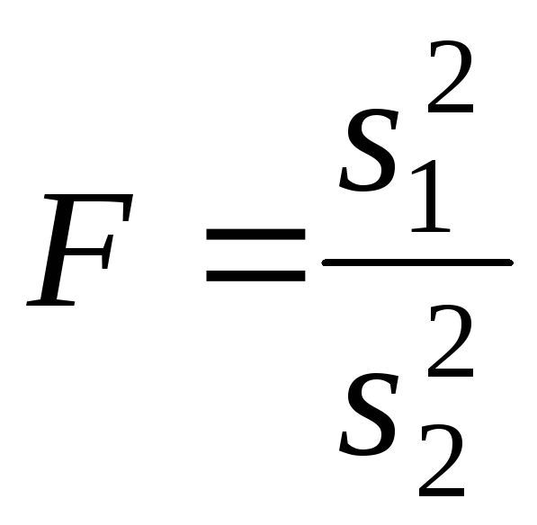 .
.
Эта величина
случайная, потому что в различных опытах
дисперсии принимают различные, наперёд
неизвестные значения, и распределена
по закону Фишера – Снедекора.
Для проверки
гипотезы по данным выборок вычисляют
частные значения входящих в критерий
величин и таким образом получают частное
(наблюдаемое) значение критерия.
Наблюдаемым
значением
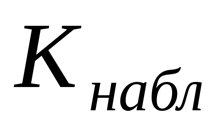 называют значение критерия, вычисленное
по выборкам. Например, если по двум
выборкам найдены исправленные выборочные
дисперсии и
и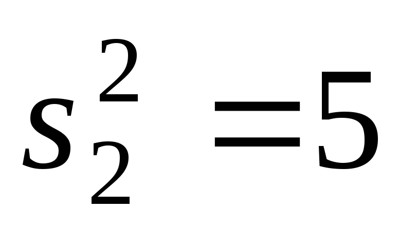 ,
,
то наблюдаемое значение критерия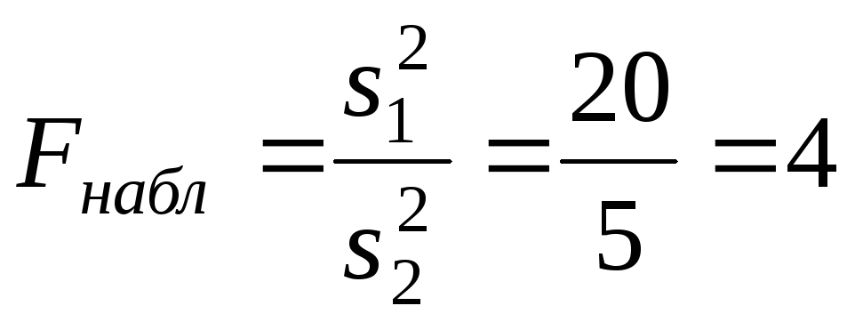 .
.
Критическая
область. Область принятия гипотезы.
Критические точки
После выбора
определённого критерия множество всех
его возможных значений разбивают на
два непересекающихся подмножества:
одно из них содержит значения критерия,
при которых нулевая гипотеза отвергается,
а другая – при которых она принимается.
Критической
областью называют совокупность значений
критерия, при которых нулевую гипотезу
отвергают.
Областью принятия
гипотезы (областью допустимых значений)
называют совокупность значений критерия,
при которых гипотезу принимают.
Основной принцип
проверки статистических гипотез можно
сформулировать так: если наблюдаемое
значение критерия принадлежит критической
области – гипотезу отвергают, если
наблюдаемое значение критерия принадлежит
области принятия гипотезы – гипотезу
принимают.
Поскольку критерий
 — одномерная случайная величина, все её
возможные значения принадлежат некоторому
интервалу. Поэтому критическая область
и область принятия гипотезы также
являются интервалами и, следовательно,
существуют точки, которые их разделяют.
Критическими
точками (границами)
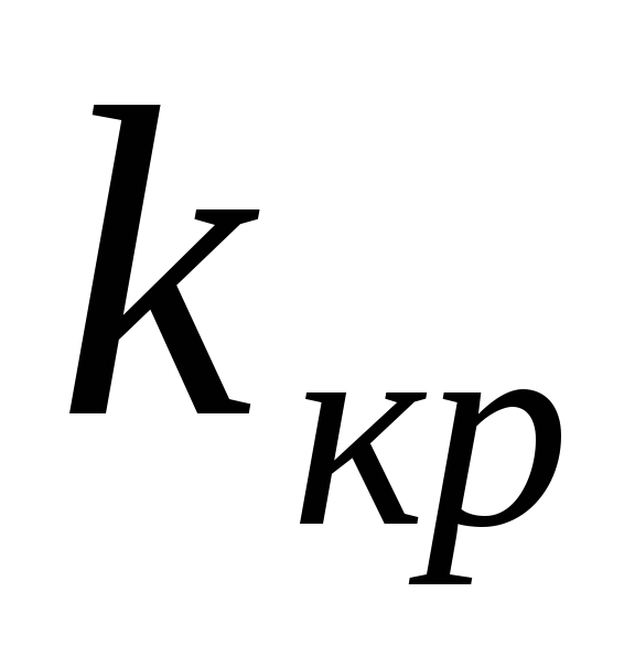 называют точки, отделяющие критическую
область от области принятия гипотезы.
Различают
одностороннюю (правостороннюю или
левостороннюю) и двустороннюю критические
области.
Правосторонней
называют критическую область, определяемую
неравенством
 >
>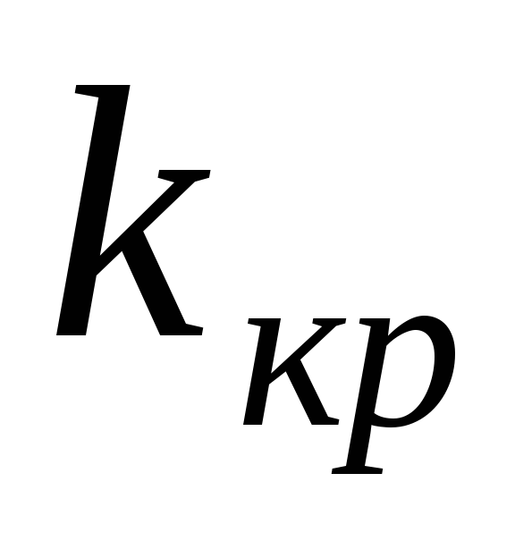 ,
,
где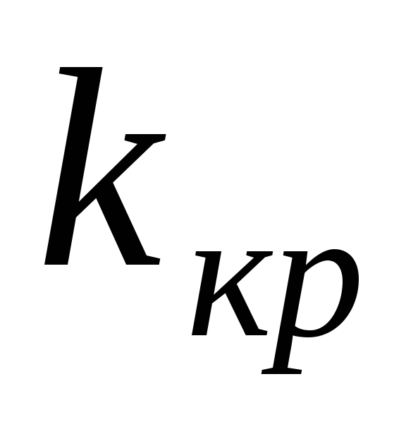 — положительное число.
Левосторонней
называют критическую область, определяемую
неравенством
 <
<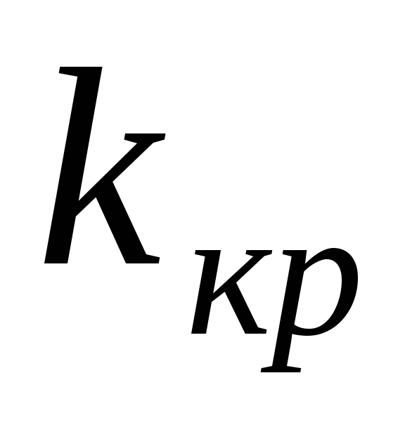 ,
,
где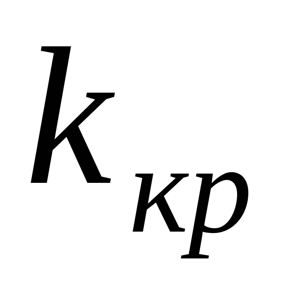 — отрицательное число.
Односторонней
называют правостороннюю или левостороннюю
критическую область.
Двусторонней
называют критическую область, определяемую
неравенствами
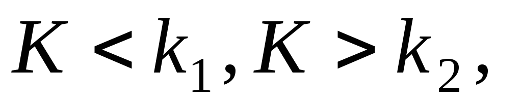 где
где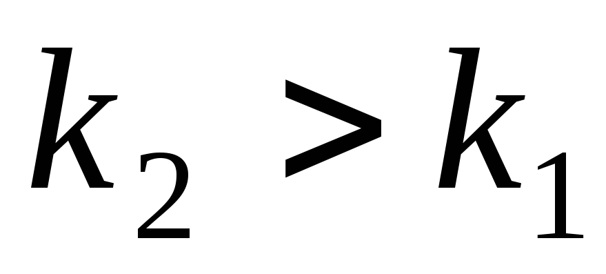 .
.
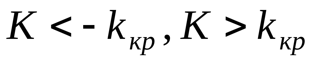
В частности, если
критические точки симметричны относительно
нуля, двусторонняя критическая область
определяется неравенствами ( в
предположении, что
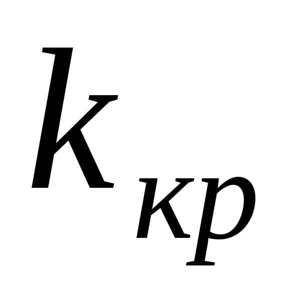 >0):
>0):
 ,
,
или равносильным неравенством
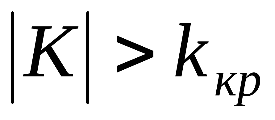 .
.
Отыскание
правосторонней критической области
Как найти критическую
область? Обоснованный ответ на этот
вопрос требует привлечения довольно
сложной теории. Ограничимся её элементами.
Для определённости начнём с нахождения
правосторонней критической области,
которая определяется неравенством
 >
>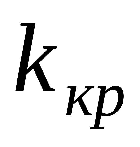 ,
,
где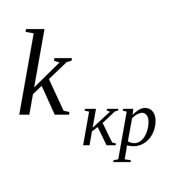 >0.
>0.
Видим, что для отыскания правосторонней
критической области достаточно найти
критическую точку. Следовательно,
возникает новый вопрос: как её найти?
Для её нахождения
задаются достаточной малой вероятностью
– уровнем значимости
 .
.
Затем ищут критическую точку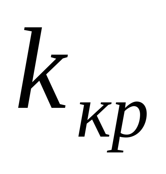 ,
,
исходя из требования, чтобы при условии
справедливости нулевой гипотезы
вероятность того, критерий примет значение, большее
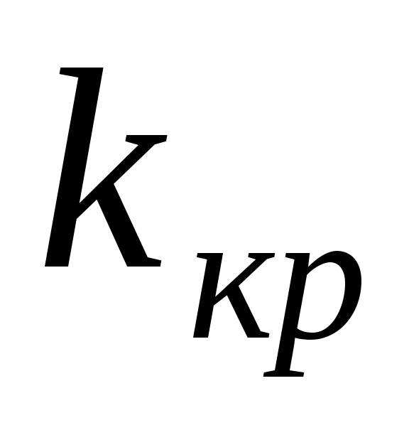 ,
,
была равна принятому уровню значимости:
Р( >
>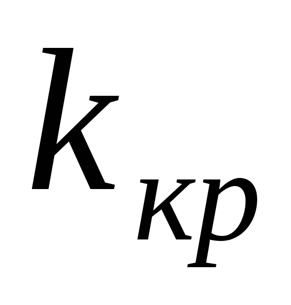 )=
)= .
.
Для каждого критерия
имеются соответствующие таблицы, по
которым и находят критическую точку,
удовлетворяющую этому требованию.
Замечание 1.
Когда
критическая точка уже найдена, вычисляют
по данным выборок наблюдаемое значение
критерия и, если окажется, что
 >
>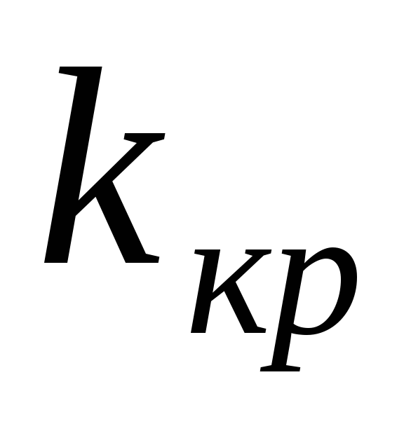 ,
,
то нулевую гипотезу отвергают; если же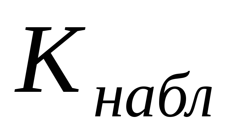 <
<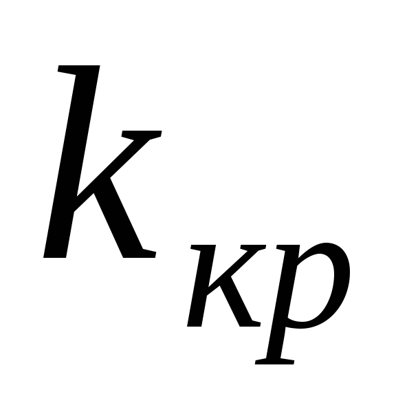 ,
,
то нет оснований, чтобы отвергнуть
нулевую гипотезу.
Пояснение. Почему
правосторонняя критическая область
была определена, исходя из требования,
чтобы при справедливости нулевой
гипотезы выполнялось соотношение
Р( >
>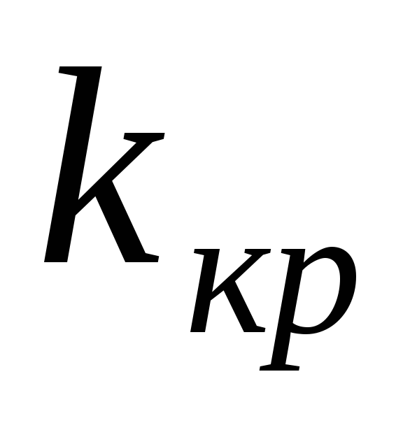 )=
)= ?
?
(*)
Поскольку вероятность
события
 >
>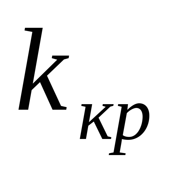 мала (
 — малая вероятность), такое событие при
справедливости нулевой гипотезы, в силу
принципа практической невозможности
маловероятных событий, в единичном
испытании не должно наступить. Если всё
же оно произошло, т.е. наблюдаемое
значение критерия оказалось больше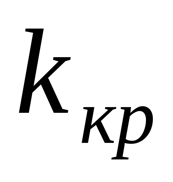 ,
,
то это можно объяснить тем, что нулевая
гипотеза ложна и, следовательно, должна
быть отвергнута. Таким образом, требование
(*) определяет такие значения критерия,
при которых нулевая гипотеза отвергается,
а они и составляют правостороннюю
критическую область.
Замечание 2.
Наблюдаемое значение критерия может
оказаться большим
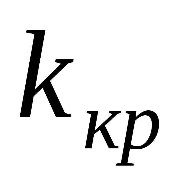 не потому, что нулевая гипотеза ложна,
а по другим причинам (малый объём выборки,
недостатки методики эксперимента и
др.). В этом случае, отвергнув правильную
нулевую гипотезу, совершают ошибку
первого рода. Вероятность этой ошибки
равна уровню значимости .
.
Итак, пользуясь требованием (*), мы с
вероятностью рискуем совершить ошибку первого рода.
Замечание 3. Пусть
нулевая гипотеза принята; ошибочно
думать, что тем самым она доказана.
Действительно, известно, что один пример,
подтверждающий справедливость некоторого
общего утверждения, ещё не доказывает
его. Поэтому более правильно говорить,
«данные наблюдений согласуются с нулевой
гипотезой и, следовательно, не дают
оснований её отвергнуть».
На практике для
большей уверенности принятия гипотезы
её проверяют другими способами или
повторяют эксперимент, увеличив объём
выборки.
Отвергают гипотезу
более категорично, чем принимают.
Действительно, известно, что достаточно
привести один пример, противоречащий
некоторому общему утверждению, чтобы
это утверждение отвергнуть. Если
оказалось, что наблюдаемое значение
критерия принадлежит критической
области, то этот факт и служит примером,
противоречащим нулевой гипотезе, что
позволяет её отклонить.
Отыскание
левосторонней и двусторонней критических
областей***
Отыскание
левосторонней и двусторонней критических
областей сводится (так же, как и для
правосторонней) к нахождению соответствующих
критических точек. Левосторонняя
критическая область определяется
неравенством
 <
<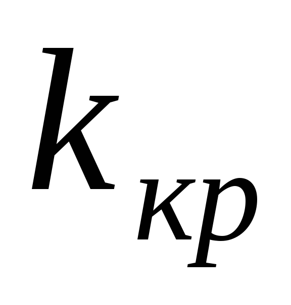 (
(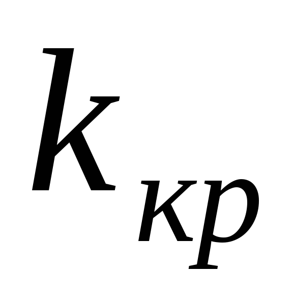 <0).
<0).
Критическую точку находят, исходя из
требования, чтобы при справедливости
нулевой гипотезы вероятность того, что
критерий примет значение, меньшее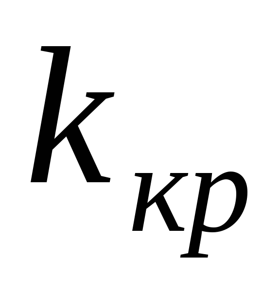 ,
,
была равна принятому уровню значимости:
Р( <
<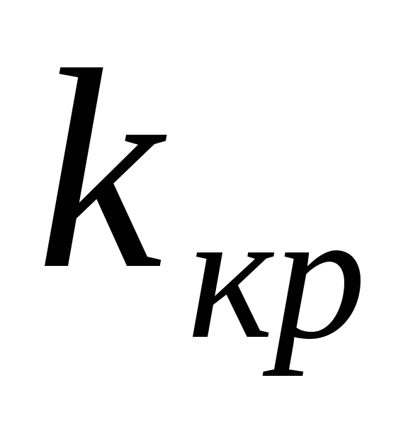 )=
)= .
.
Двусторонняя
критическая область определяется
неравенствами
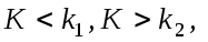 Критические
точки находят, исходя из требования,
чтобы при справедливости нулевой
гипотезы сумма вероятностей того, что
критерий примет значение, меньшее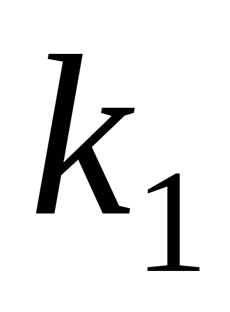 или большее
 ,
,
была равна принятому уровню значимости:
 .
.
(*)
Ясно, что критические
точки могут быть выбраны бесчисленным
множеством способов. Если же распределение
критерия симметрично относительно нуля
и имеются основания (например, для
увеличения мощности) выбрать симметричные
относительно нуля точки (-
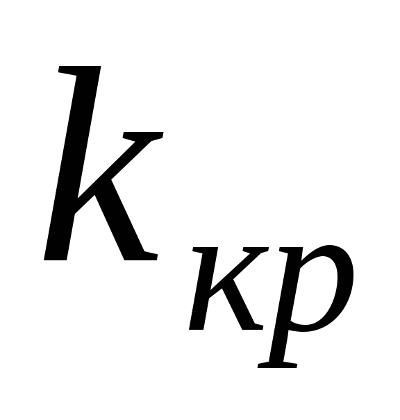 )и
)и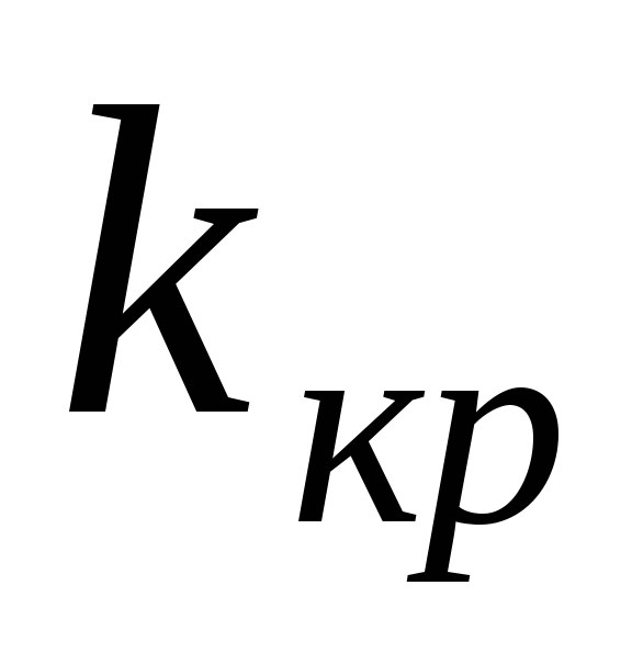 (
(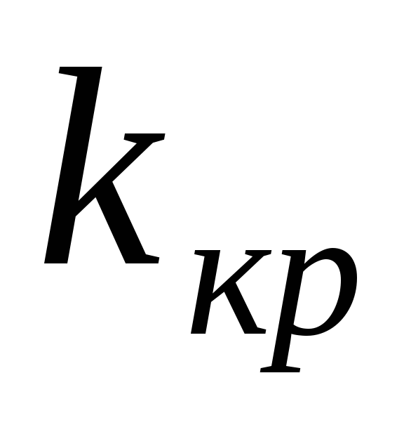 >0),
>0),
то
 Учитывая (*), получим
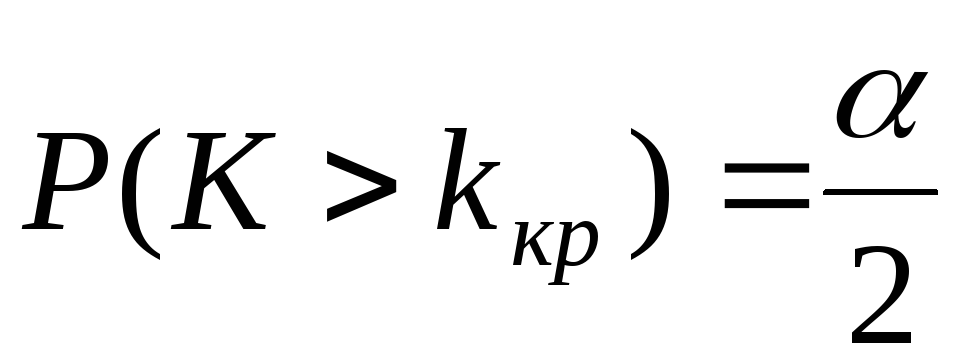 .
.
Это соотношение
и служит для отыскания критических
точек двусторонней критической области.
Критические точки находят по соответствующим
таблицам.
Дополнительные
сведения о выборе критической области.
Мощность критерия
Мы строили
критическую область, исходя из требования,
чтобы вероятность попадания в неё
критерия была равна
 при условии, что нулевая гипотеза
справедлива. Оказывается целесообразным
ввести в рассмотрение вероятность
попадания критерия в критическую область
при условии, что нулевая гипотеза неверна
и, следовательно, справедлива конкурирующая.
Мощностью критерия
называют вероятность попадания критерия
в критическую область при условии, что
справедлива конкурирующая гипотеза.
Другими словами, мощность критерия есть
вероятность того, что нулевая гипотеза
будет отвергнута, если верна конкурирующая
гипотеза.
Пусть для проверки
гипотезы принят определённый уровень
значимости и выборка имеет фиксированный
объём. Остаётся произвол в выборе
критической области. Покажем, что её
целесообразно построить так, чтобы
мощность критерия была максимальной.
Предварительно убедимся, что если
вероятность ошибки второго рода (принять
неправильную гипотезу) равна
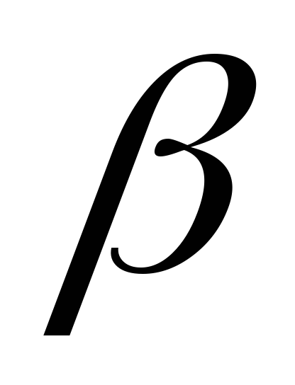 ,
,
то мощность равна 1-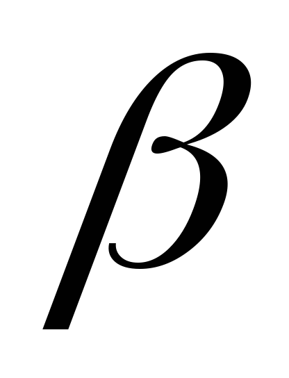 .
.
Действительно, если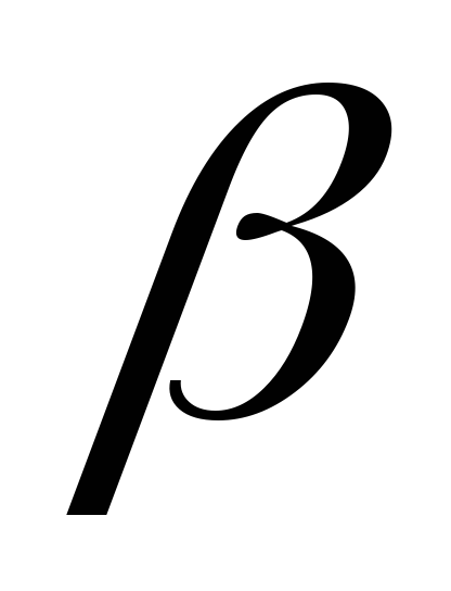 — вероятность ошибки второго рода, т.е.
события «принята нулевая гипотеза,
причём справедливо конкурирующая», то
мощность критерия равна 1 —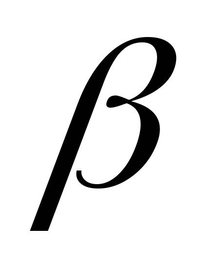 .
.
Пусть мощность 1
—
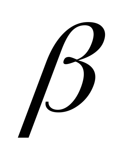 возрастает; следовательно, уменьшается
вероятность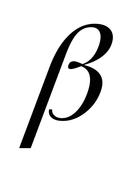 совершить ошибку второго рода. Таким
образом, чем мощность больше, тем
вероятность ошибки второго рода меньше.
Итак, если уровень
значимости уже выбран, то критическую
область следует строить так, чтобы
мощность критерия была максимальной.
Выполнение этого требования должно
обеспечить минимальную ошибку второго
рода, что, конечно, желательно.
Замечание 1.
Поскольку вероятность события «ошибка
второго рода допущена» равна
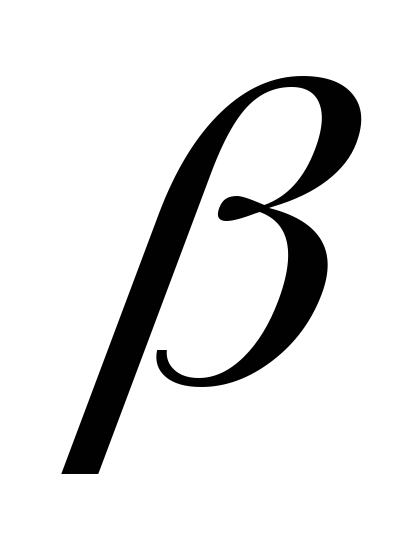 ,
,
то вероятность противоположного события
«ошибка второго рода не допущена» равна
1 —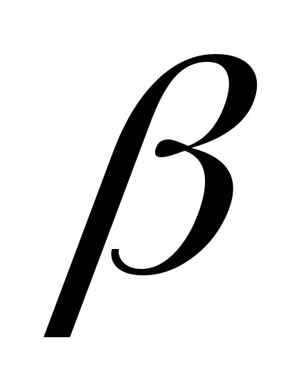 ,
,
т.е. мощности критерия. Отсюда следует,
что мощность критерия есть вероятность
того, что не будет допущена ошибка
второго рода.
Замечание 2. Ясно,
что чем меньше вероятности ошибок
первого и второго рода, тем критическая
область «лучше». Однако при заданном
объёме выборки уменьшить одновременно
 и
и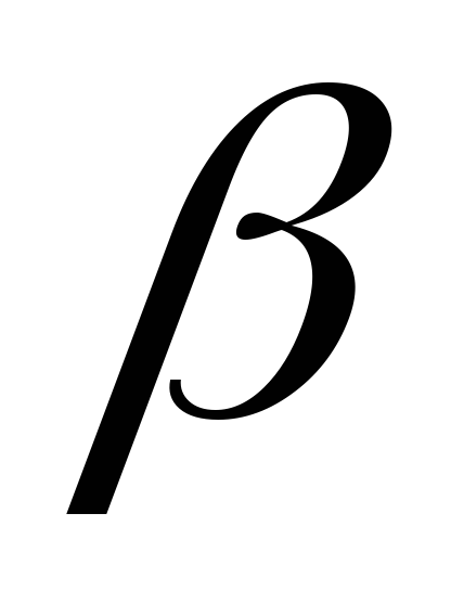 невозможно; если уменьшить
 ,
,
то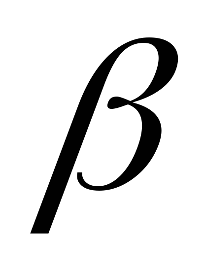 будет возрастать. Например, если принять
 =0,
=0,
то будут приниматься все гипотезы, в
том числе и неправильные, т.е. возрастает
вероятность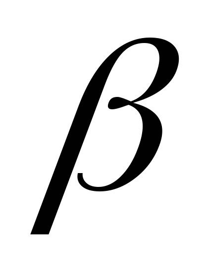 ошибки второго рода.
Как же выбрать
 наиболее целесообразно? Ответ на этот
вопрос зависит от «тяжести последствий»
ошибок для каждой конкретной задачи.
Например, если ошибка первого рода
повлечёт большие потери, а второго рода
– малые, то следует принять возможно
меньшее .
.
Если
 уже выбрано, то, пользуясь теоремой Ю.
Неймана и Э.Пирсона, можно построить
критическую область, для которой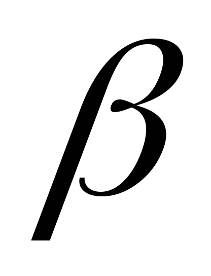 будет минимальным и, следовательно,
мощность критерия максимальной.
Замечание 3.
Единственный способ одновременного
уменьшения вероятностей ошибок первого
и второго рода состоит в увеличении
объёма выборок.
Соседние файлы в папке Лекции 2 семестр
- #
- #
- #
- #
Ошибки I и II рода при проверке гипотез, мощность
Общий обзор
Принятие неправильного решения
Мощность и связанные факторы
Проверка множественных гипотез
Общий обзор
Большинство проверяемых гипотез сравнивают между собой группы объектов, которые испытывают влияние различных факторов.
Например, можно сравнить эффективность двух видов лечения, чтобы сократить 5-летнюю смертность от рака молочной железы. Для данного исхода (например, смерть) сравнение, представляющее интерес (например, различные показатели смертности через 5 лет), называют эффектом или, если уместно, эффектом лечения.
Нулевую гипотезу выражают как отсутствие эффекта (например 5-летняя смертность от рака молочной железы одинаковая в двух группах, получающих разное лечение); двусторонняя альтернативная гипотеза будет означать, что различие эффектов не равно нулю.
Критериальная проверка гипотезы дает возможность определить, достаточно ли аргументов, чтобы отвергнуть нулевую гипотезу. Можно принять только одно из двух решений:
- отвергнуть нулевую гипотезу и принять альтернативную гипотезу
- остаться в рамках нулевой гипотезы
Важно: В литературе достаточно часто встречается понятие «принять нулевую гипотезу». Хотелось бы внести ясность, что со статистической точки зрения принять нулевую гипотезу невозможно, т.к. нулевая гипотеза представляет собой достаточно строгое утверждение (например, средние значения в сравниваемых группах равны  ).
).
Поэтому фразу о принятии нулевой гипотезы следует понимать как то, что мы просто остаемся в рамках гипотезы.
Принятие неправильного решения
Возможно неправильное решение, когда отвергают/не отвергают нулевую гипотезу, потому что есть только выборочная информация.
| |
Верная гипотеза | ||
|---|---|---|---|
| H0 | H1 | ||
| Результат применения критерия |
H0 | H0 верно принята | H0 неверно принята (Ошибка второго рода) |
| H1 | H0 неверно отвергнута (Ошибка первого рода) |
H0 верно отвергнута |
Ошибка 1-го рода: нулевую гипотезу отвергают, когда она истинна, и делают вывод, что имеется эффект, когда в действительности его нет. Максимальный шанс (вероятность) допустить ошибку 1-го рода обозначается α (альфа). Это уровень значимости критерия; нулевую гипотезу отвергают, если наше значение p ниже уровня значимости, т. е., если p < α.
Следует принять решение относительно значения а прежде, чем будут собраны данные; обычно назначают условное значение 0,05, хотя можно выбрать более ограничивающее значение, например 0,01.
Шанс допустить ошибку 1-го рода никогда не превысит выбранного уровня значимости, скажем α = 0,05, так как нулевую гипотезу отвергают только тогда, когда p< 0,05. Если обнаружено, что p > 0,05, то нулевую гипотезу не отвергнут и, следовательно, не допустят ошибки 1-го рода.
Ошибка 2-го рода: не отвергают нулевую гипотезу, когда она ложна, и делают вывод, что нет эффекта, тогда как в действительности он существует. Шанс возникновения ошибки 2-го рода обозначается β (бета); а величина (1-β) называется мощностью критерия.
Следовательно, мощность — это вероятность отклонения нулевой гипотезы, когда она ложна, т.е. это шанс (обычно выраженный в процентах) обнаружить реальный эффект лечения в выборке данного объема как статистически значимый.
В идеале хотелось бы, чтобы мощность критерия составляла 100%; однако это невозможно, так как всегда остается шанс, хотя и незначительный, допустить ошибку 2-го рода.
К счастью, известно, какие факторы влияют на мощность и, таким образом, можно контролировать мощность критерия, рассматривая их.
Мощность и связанные факторы
Планируя исследование, необходимо знать мощность предложенного критерия. Очевидно, можно начинать исследование, если есть «хороший» шанс обнаружить уместный эффект, если таковой существует (под «хорошим» мы подразумеваем, что мощность должна быть по крайней мере 70-80%).
Этически безответственно начинать исследование, у которого, скажем, только 40% вероятности обнаружить реальный эффект лечения; это бесполезная трата времени и денежных средств.
Ряд факторов имеют прямое отношение к мощности критерия.
Объем выборки: мощность критерия увеличивается по мере увеличения объема выборки. Это означает, что у большей выборки больше возможностей, чем у незначительной, обнаружить важный эффект, если он существует.
Когда объем выборки небольшой, у критерия может быть недостаточно мощности, чтобы обнаружить отдельный эффект. Эти методы также можно использовать для оценки мощности критерия для точно установленного объема выборки.
Вариабельность наблюдений: мощность увеличивается по мере того, как вариабельность наблюдений уменьшается.
Интересующий исследователя эффект: мощность критерия больше для более высоких эффектов. Критерий проверки гипотез имеет больше шансов обнаружить значительный реальный эффект, чем незначительный.
Уровень значимости: мощность будет больше, если уровень значимости выше (это эквивалентно увеличению допущения ошибки 1-го рода, α, а допущение ошибки 2-го рода, β, уменьшается).
Таким образом, вероятнее всего, исследователь обнаружит реальный эффект, если на стадии планирования решит, что будет рассматривать значение р как значимое, если оно скорее будет меньше 0,05, чем меньше 0,01.
Обратите внимание, что проверка ДИ для интересующего эффекта указывает на то, была ли мощность адекватной. Большой доверительный интервал следует из небольшой выборки и/или набора данных с существенной вариабельностью и указывает на недостаточную мощность.
Проверка множественных гипотез
Часто нужно выполнить критериальную проверку значимости множественных гипотез на наборе данных с многими переменными или существует более двух видов лечения.
Ошибка 1-го рода драматически увеличивается по мере увеличения числа сравнений, что приводит к ложным выводам относительно гипотез. Следовательно, следует проверить только небольшое число гипотез, выбранных для достижения первоначальной цели исследования и точно установленных априорно.
Можно использовать какую-нибудь форму апостериорного уточнения значения р, принимая во внимание число выполненных проверок гипотез.
Например, при подходе Бонферрони (его часто считают довольно консервативным) умножают каждое значение р на число выполненных проверок; тогда любые решения относительно значимости будут основываться на этом уточненном значении р.
Связанные определения:
p-уровень
Альтернативная гипотеза, альтернатива
Альфа-уровень
Бета-уровень
Гипотеза
Двусторонний критерий
Критерий для проверки гипотезы
Критическая область проверки гипотезы
Мощность
Мощность исследования
Мощность статистического критерия
Нулевая гипотеза
Односторонний критерий
Ошибка I рода
Ошибка II рода
Статистика критерия
Эквивалентные статистические критерии
В начало
Содержание портала
Содержание
- Ошибки I и II рода при проверке гипотез, мощность
- Общий обзор
- Принятие неправильного решения
- Мощность и связанные факторы
- Проверка множественных гипотез
- Виды ошибок при проверке гипотез
- Введение в проверку гипотез
- Два типа статистических гипотез
- Проверка гипотез
- Два типа ошибок принятия решений
- Односторонний и двусторонний тесты
- Раздел 2 лекция 5
Ошибки I и II рода при проверке гипотез, мощность
Общий обзор
Большинство проверяемых гипотез сравнивают между собой группы объектов, которые испытывают влияние различных факторов.
Например, можно сравнить эффективность двух видов лечения, чтобы сократить 5-летнюю смертность от рака молочной железы. Для данного исхода (например, смерть) сравнение, представляющее интерес (например, различные показатели смертности через 5 лет), называют эффектом или, если уместно, эффектом лечения.
Нулевую гипотезу выражают как отсутствие эффекта (например 5-летняя смертность от рака молочной железы одинаковая в двух группах, получающих разное лечение); двусторонняя альтернативная гипотеза будет означать, что различие эффектов не равно нулю.
Критериальная проверка гипотезы дает возможность определить, достаточно ли аргументов, чтобы отвергнуть нулевую гипотезу. Можно принять только одно из двух решений:
- отвергнуть нулевую гипотезу и принять альтернативную гипотезу
- остаться в рамках нулевой гипотезы
Важно: В литературе достаточно часто встречается понятие «принять нулевую гипотезу». Хотелось бы внести ясность, что со статистической точки зрения принять нулевую гипотезу невозможно, т.к. нулевая гипотеза представляет собой достаточно строгое утверждение (например, средние значения в сравниваемых группах равны ).
Поэтому фразу о принятии нулевой гипотезы следует понимать как то, что мы просто остаемся в рамках гипотезы.
Принятие неправильного решения
Возможно неправильное решение, когда отвергают/не отвергают нулевую гипотезу, потому что есть только выборочная информация.
| Верная гипотеза | |||
|---|---|---|---|
| H | H1 | ||
| Результат применения критерия |
H | H верно принята | H неверно принята (Ошибка второго рода) |
| H1 | H неверно отвергнута (Ошибка первого рода) |
H верно отвергнута |
Ошибка 1-го рода: нулевую гипотезу отвергают, когда она истинна, и делают вывод, что имеется эффект, когда в действительности его нет. Максимальный шанс (вероятность) допустить ошибку 1-го рода обозначается α (альфа). Это уровень значимости критерия; нулевую гипотезу отвергают, если наше значение p ниже уровня значимости, т. е., если p 0,05, то нулевую гипотезу не отвергнут и, следовательно, не допустят ошибки 1-го рода.
Ошибка 2-го рода: не отвергают нулевую гипотезу, когда она ложна, и делают вывод, что нет эффекта, тогда как в действительности он существует. Шанс возникновения ошибки 2-го рода обозначается β (бета); а величина (1-β) называется мощностью критерия.
Следовательно, мощность — это вероятность отклонения нулевой гипотезы, когда она ложна, т.е. это шанс (обычно выраженный в процентах) обнаружить реальный эффект лечения в выборке данного объема как статистически значимый.
В идеале хотелось бы, чтобы мощность критерия составляла 100%; однако это невозможно, так как всегда остается шанс, хотя и незначительный, допустить ошибку 2-го рода.
К счастью, известно, какие факторы влияют на мощность и, таким образом, можно контролировать мощность критерия, рассматривая их.
Мощность и связанные факторы
Планируя исследование, необходимо знать мощность предложенного критерия. Очевидно, можно начинать исследование, если есть «хороший» шанс обнаружить уместный эффект, если таковой существует (под «хорошим» мы подразумеваем, что мощность должна быть по крайней мере 70-80%).
Этически безответственно начинать исследование, у которого, скажем, только 40% вероятности обнаружить реальный эффект лечения; это бесполезная трата времени и денежных средств.
Ряд факторов имеют прямое отношение к мощности критерия.
Объем выборки: мощность критерия увеличивается по мере увеличения объема выборки. Это означает, что у большей выборки больше возможностей, чем у незначительной, обнаружить важный эффект, если он существует.
Когда объем выборки небольшой, у критерия может быть недостаточно мощности, чтобы обнаружить отдельный эффект. Эти методы также можно использовать для оценки мощности критерия для точно установленного объема выборки.
Вариабельность наблюдений: мощность увеличивается по мере того, как вариабельность наблюдений уменьшается.
Интересующий исследователя эффект: мощность критерия больше для более высоких эффектов. Критерий проверки гипотез имеет больше шансов обнаружить значительный реальный эффект, чем незначительный.
Уровень значимости: мощность будет больше, если уровень значимости выше (это эквивалентно увеличению допущения ошибки 1-го рода, α, а допущение ошибки 2-го рода, β, уменьшается).
Таким образом, вероятнее всего, исследователь обнаружит реальный эффект, если на стадии планирования решит, что будет рассматривать значение р как значимое, если оно скорее будет меньше 0,05, чем меньше 0,01.
Обратите внимание, что проверка ДИ для интересующего эффекта указывает на то, была ли мощность адекватной. Большой доверительный интервал следует из небольшой выборки и/или набора данных с существенной вариабельностью и указывает на недостаточную мощность.
Проверка множественных гипотез
Часто нужно выполнить критериальную проверку значимости множественных гипотез на наборе данных с многими переменными или существует более двух видов лечения.
Ошибка 1-го рода драматически увеличивается по мере увеличения числа сравнений, что приводит к ложным выводам относительно гипотез. Следовательно, следует проверить только небольшое число гипотез, выбранных для достижения первоначальной цели исследования и точно установленных априорно.
Можно использовать какую-нибудь форму апостериорного уточнения значения р, принимая во внимание число выполненных проверок гипотез.
Например, при подходе Бонферрони (его часто считают довольно консервативным) умножают каждое значение р на число выполненных проверок; тогда любые решения относительно значимости будут основываться на этом уточненном значении р.
Источник
Виды ошибок при проверке гипотез


1) Ошибка первого рода.
Нулевая гипотеза H отвергается, хотя является верной. Вероятность совершения такой ошибки равна  .
.
2) Ошибка второго рода.
Нулевая гипотеза H принимается, хотя является неверной. Вероятность совершения этой ошибки равна 1 —  . Здесь — вероятность того, что ошибка второго рода не будет допущена (так называемая мощность критерия).
Пусть, например, нулевая гипотеза H означает, что определенная партия товаров соответствует условиям поставки. Если эта партия отклоняется, хотя гипотеза соответствуетдействительности, то совершается ошибка первого рода. В таком случае говорят о риске производителя товаров. Если же партия принимается, хотя она и не соответствует условиям поставки, то имеет место ошибка второго рода (так называемый риск потребителя).
Глава 1 Макроэкономичекое планирование и прогнозированиев системе регулирования социальногорыночного хозяйства
Источник
Введение в проверку гипотез
Статистическая гипотеза – это предположение о параметре совокупности .
Например, мы можем предположить, что средний рост мужчины в США составляет 70 дюймов.
Предположение о росте является статистической гипотезой , а истинный средний рост мужчины в США является популяционным параметром .
Проверка гипотезы — это формальный статистический тест, который мы используем, чтобы отвергнуть или не опровергнуть статистическую гипотезу.
Два типа статистических гипотез
Чтобы проверить, верна ли статистическая гипотеза о параметре совокупности, мы получаем случайную выборку из совокупности и выполняем проверку гипотезы на выборочных данных.
Существует два типа статистических гипотез:
Нулевая гипотеза , обозначаемая как H 0 , представляет собой гипотезу о том, что выборка данных происходит чисто случайно.
Альтернативная гипотеза , обозначаемая как H 1 или H a , представляет собой гипотезу о том, что на выборочные данные влияет какая-то неслучайная причина.
Проверка гипотез
Проверка гипотезы состоит из пяти шагов:
1. Сформулируйте гипотезы.
Сформулируйте нулевую и альтернативную гипотезы. Эти две гипотезы должны быть взаимоисключающими, поэтому, если одна верна, другая должна быть ложной.
2. Определите уровень значимости для гипотезы.
Определите уровень значимости. Распространенные варианты: .01, .05 и .1.
3. Найдите тестовую статистику.
Найдите тестовую статистику и соответствующее значение p. Часто мы анализируем среднее значение или долю населения, и общая формула для нахождения тестовой статистики выглядит следующим образом: (выборочная статистика — параметр совокупности) / (стандартное отклонение статистики)
4. Отклонить или не отклонить нулевую гипотезу.
Используя тестовую статистику или p-значение, определите, можете ли вы отклонить или не отклонить нулевую гипотезу на основе уровня значимости.
Значение p говорит нам о силе доказательств в поддержку нулевой гипотезы. Если p-значение меньше уровня значимости, мы отклоняем нулевую гипотезу.
5. Интерпретируйте результаты.
Интерпретируйте результаты проверки гипотезы в контексте заданного вопроса.
Два типа ошибок принятия решений
Есть два типа ошибок принятия решений, которые можно сделать при проверке гипотезы:
Ошибка I типа: вы отвергаете нулевую гипотезу, когда она на самом деле верна. Вероятность совершения ошибки первого рода равна уровню значимости, часто называемому альфа и обозначаемому как α.
Ошибка типа II: вы не можете отвергнуть нулевую гипотезу, когда она на самом деле ложна. Вероятность совершения ошибки типа II называется мощностью теста или бета и обозначается как β.
Односторонний и двусторонний тесты
Статистическая гипотеза может быть односторонней или двусторонней.
Односторонняя гипотеза предполагает утверждение «больше» или «меньше».
Например, предположим, что средний рост мужчины в США больше или равен 70 дюймам. Нулевой гипотезой будет H0: µ ≥ 70 дюймов, а альтернативной гипотезой будет Ha: µ
Источник
Раздел 2 лекция 5
Раздел 2 Статистические гипотезы и их проверка
Тема: общие принципы проверки статистических гипотез.
План: 1.Понятие статистической гипотезы. Ошибки I и II рода.
2.Критерий оценки статистических гипотез. Уровень значимости.
Понятие статистической гипотезы. Ошибки I и II рода.
Статистической гипотезой называется предположение о том, что распределение случайной величины (результата эксперимента) подчиняется определённому закону распределения.
Статистический критерий (или критерий оценки статистической гипотезы) -это проверка, позволяющая оценить, насколько статистическая гипотеза согласуется с экспериментальными данными.
Пусть в нашем распоряжении имеется величина х – одно из возможных значений случайной величины (результата эксперимента).
Выдвинем гипотезу о том, что случайная величина х распределена по закону, задаваемому функцией плотности вероятности φ(х). Гипотезу обозначим как Н и назовем нуль гипотезой.
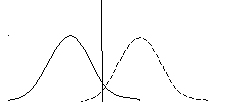
Введём также некоторую альтернативную гипотезу Н1, содержание которой состоит в том, что рассматриваемая случайная величина х подчиняется закону распределения, описываемого функцией плотности вероятности φ1(х). Будем считать, что гипотеза Н1 является истинной, если нуль-гипотеза Н не верна. Требуется на основании распределения величины х решить, какой из гипотез Н или Н1 следует отдать предпочтение. Решение поставленной задачи может быть как верным, так и ложным.
Неправильное решение может быть двух родов:
Ошибка первого рода – не принять нуль-гипотезу, когда она в действительности верна, (т.е принять Н1 вместо Н). α – это вероятность совершить ошибку I рода (или риск) – показывает какова вероятность отбросить верные (истинные) результаты.
Ошибка второго рода – принять нуль-гипотезу, когда она не верна (т.е. принять Н вместо Н1 ). β – это вероятность совершить ошибку второго рода. Показывает какова вероятность принять неверные (ложные) результаты.
Тогда, α уменьшается, β увеличивается, а (1–β) уменьшается. Т.е. α уменьшается (вероятность не принять Н, когда она верна) следовательно (1- β) уменьшается (вероятность не принять, когда Н не верна).
Поэтому, для принятия проверяемой гипотезы вероятность совершить ошибку I рода α должна быть не самой низкой, а оптимальной.
Для выбора величины α существуют определённые правила (критерии), которые позволяют оценить насколько верно проверяемая гипотеза описывает экспериментальные данные.
Критерии оценки статистических гипотез при обработке результатов эксперимента
Рассмотрим критерии оценки гипотезы Н (т.е. верна она или нет) для случайной величины х (т.е. для результата эксперимента). Пусть гипотеза Н верна и состоит в том, что рассматриваемая случайная величина х действительно распределена по закону, задаваемому функцией φ(х). Однако, если х попало в область, расположенную вблизи правого или левого «хвоста» функции φ(х), то вероятность попадания случайной величины в эту область, вычисляется при помощи функции φ(х) мала и приближается к нулю. Поэтому проще и целесообразнее признать ошибочность гипотезы и не принять её в этой область. Тогда эта область будет характеризоваться α — вероятностью не принять гипотезу Н , когда она в действительности верна.

критическая область доверительный интервал критическая область
Назовём интервал значений случайной величины х, т.е отрезок оси абсцисс, расположенный вблизи «хвоста» функции φ(х) критической областью данной функции распределения.
Значения случайной величины х1 и х2, отделяющих критические области, называются критическими значениями данной функции распределения.
Размеры критической области определяются вероятностью попадания в неё случайных величин. Вероятность попадания значений х случайной величины в критическую область получила название уровень значимости критерия оценки статистической гипотезы или просто уровень значимости р. Видно, что
Уровень значимости (риск) – это вероятность отвергнуть проверяемую гипотезу Н, когда она в действительности верна. Проще говоря р – это вероятность отбросить верные результаты.
Критерием оценки статистической гипотезы является попадание хi в критическую область. Если случайная величина х не попадает в критическую область, то анализируемая гипотеза считается приемлемой. Если случайная величина х попадает в критическую область, то это свидетельствует о неприемлемости анализируемой гипотезы.
Если критическая область, попадание в которую значений х случайной величины, целиком расположена в правой (или левой) части графика φ(х), то критерий оценки статистической гипотезы называется односторонним. В случае одностороннего критерия уровень значимости равен α=р=(1 –Р).

 φ(х) φ(х)
В  противном случае критическую область необходимо рассматривать из двух частей, а соответственный критерий называется двухсторонним. В случае двухстороннего критерия α=р=(1 –Р)/2.
Односторонний критерий используют только в том случае, если экспериментатор заранее знает, что результаты опытов не попадают в противоположную часть (область) функции, или для него это будет иметь практическое значение.
Пример 1: 
 φ(х)
φ(х)
 +Wвлаги
Пример 2: Д окрашивание раствора
-0,16 не имеет практического значения, т.к. раствор мутный и луч не проходит через раствор – результат не верен.


 α=р=(1-Р)/2
Принять проверяемую гипотезу можно только при определённых значениях р. Критерии принятия статистической гипотезы:
Если значения уровня значимости р равно 5% и более, то проверяемую гипотезу следует признать согласующейся с полученными экспериментальными данными. В этом случае различия между гипотетическими экспериментальными данными являются статистически незначимым.
Если уровень значимости менее 5%, но более 1%, то можно пойти на риск принятия проверяемой гипотезы, либо взять гипотезу под сомнение. Различие между гипотетическими и экспериментальными данными является спорным. Для уточнения выводов следует признать целесообразным повторение эксперимента
Если значение критерия значимости составляет 1% и менее, то проверяемая гипотеза отбрасывается. Различия между гипотетическими и экспериментальными данными являются статистически значимыми.
Источник
This article is about erroneous outcomes of statistical tests. For closely related concepts in binary classification and testing generally, see false positives and false negatives.
In statistical hypothesis testing, a type I error is the mistaken rejection of an actually true null hypothesis (also known as a «false positive» finding or conclusion; example: «an innocent person is convicted»), while a type II error is the failure to reject a null hypothesis that is actually false (also known as a «false negative» finding or conclusion; example: «a guilty person is not convicted»).[1] Much of statistical theory revolves around the minimization of one or both of these errors, though the complete elimination of either is a statistical impossibility if the outcome is not determined by a known, observable causal process.
By selecting a low threshold (cut-off) value and modifying the alpha (α) level, the quality of the hypothesis test can be increased.[2] The knowledge of type I errors and type II errors is widely used in medical science, biometrics and computer science.[clarification needed]
Intuitively, type I errors can be thought of as errors of commission, i.e. the researcher unluckily concludes that something is the fact. For instance, consider a study where researchers compare a drug with a placebo. If the patients who are given the drug get better than the patients given the placebo by chance, it may appear that the drug is effective, but in fact the conclusion is incorrect.
In reverse, type II errors are errors of omission. In the example above, if the patients who got the drug did not get better at a higher rate than the ones who got the placebo, but this was a random fluke, that would be a type II error. The consequence of a type II error depends on the size and direction of the missed determination and the circumstances. An expensive cure for one in a million patients may be inconsequential even if it truly is a cure.
Definition[edit]
Statistical background[edit]
In statistical test theory, the notion of a statistical error is an integral part of hypothesis testing. The test goes about choosing about two competing propositions called null hypothesis, denoted by H0 and alternative hypothesis, denoted by H1. This is conceptually similar to the judgement in a court trial. The null hypothesis corresponds to the position of the defendant: just as he is presumed to be innocent until proven guilty, so is the null hypothesis presumed to be true until the data provide convincing evidence against it. The alternative hypothesis corresponds to the position against the defendant. Specifically, the null hypothesis also involves the absence of a difference or the absence of an association. Thus, the null hypothesis can never be that there is a difference or an association.
If the result of the test corresponds with reality, then a correct decision has been made. However, if the result of the test does not correspond with reality, then an error has occurred. There are two situations in which the decision is wrong. The null hypothesis may be true, whereas we reject H0. On the other hand, the alternative hypothesis H1 may be true, whereas we do not reject H0. Two types of error are distinguished: type I error and type II error.[3]
Type I error[edit]
The first kind of error is the mistaken rejection of a null hypothesis as the result of a test procedure. This kind of error is called a type I error (false positive) and is sometimes called an error of the first kind. In terms of the courtroom example, a type I error corresponds to convicting an innocent defendant.
Type II error[edit]
The second kind of error is the mistaken failure to reject the null hypothesis as the result of a test procedure. This sort of error is called a type II error (false negative) and is also referred to as an error of the second kind. In terms of the courtroom example, a type II error corresponds to acquitting a criminal.[4]
Crossover error rate[edit]
The crossover error rate (CER) is the point at which type I errors and type II errors are equal. A system with a lower CER value provides more accuracy than a system with a higher CER value.
False positive and false negative[edit]
In terms of false positives and false negatives, a positive result corresponds to rejecting the null hypothesis, while a negative result corresponds to failing to reject the null hypothesis; «false» means the conclusion drawn is incorrect. Thus, a type I error is equivalent to a false positive, and a type II error is equivalent to a false negative.
Table of error types[edit]
Tabularised relations between truth/falseness of the null hypothesis and outcomes of the test:[5]
| Table of error types | Null hypothesis (H0) is |
||
|---|---|---|---|
| True | False | ||
| Decision about null hypothesis (H0) |
Don’t reject |
Correct inference (true negative) (probability = 1−α) |
Type II error (false negative) (probability = β) |
| Reject | Type I error (false positive) (probability = α) |
Correct inference (true positive) (probability = 1−β) |
Error rate[edit]

The results obtained from negative sample (left curve) overlap with the results obtained from positive samples (right curve). By moving the result cutoff value (vertical bar), the rate of false positives (FP) can be decreased, at the cost of raising the number of false negatives (FN), or vice versa (TP = True Positives, TPR = True Positive Rate, FPR = False Positive Rate, TN = True Negatives).
A perfect test would have zero false positives and zero false negatives. However, statistical methods are probabilistic, and it cannot be known for certain whether statistical conclusions are correct. Whenever there is uncertainty, there is the possibility of making an error. Considering this nature of statistics science, all statistical hypothesis tests have a probability of making type I and type II errors.[6]
- The type I error rate is the probability of rejecting the null hypothesis given that it is true. The test is designed to keep the type I error rate below a prespecified bound called the significance level, usually denoted by the Greek letter α (alpha) and is also called the alpha level. Usually, the significance level is set to 0.05 (5%), implying that it is acceptable to have a 5% probability of incorrectly rejecting the true null hypothesis.[7]
- The rate of the type II error is denoted by the Greek letter β (beta) and related to the power of a test, which equals 1−β.[8]
These two types of error rates are traded off against each other: for any given sample set, the effort to reduce one type of error generally results in increasing the other type of error.[9]
The quality of hypothesis test[edit]
The same idea can be expressed in terms of the rate of correct results and therefore used to minimize error rates and improve the quality of hypothesis test. To reduce the probability of committing a type I error, making the alpha value more stringent is quite simple and efficient. To decrease the probability of committing a type II error, which is closely associated with analyses’ power, either increasing the test’s sample size or relaxing the alpha level could increase the analyses’ power.[10] A test statistic is robust if the type I error rate is controlled.
Varying different threshold (cut-off) value could also be used to make the test either more specific or more sensitive, which in turn elevates the test quality. For example, imagine a medical test, in which an experimenter might measure the concentration of a certain protein in the blood sample. The experimenter could adjust the threshold (black vertical line in the figure) and people would be diagnosed as having diseases if any number is detected above this certain threshold. According to the image, changing the threshold would result in changes in false positives and false negatives, corresponding to movement on the curve.[11]
Example[edit]
Since in a real experiment it is impossible to avoid all type I and type II errors, it is important to consider the amount of risk one is willing to take to falsely reject H0 or accept H0. The solution to this question would be to report the p-value or significance level α of the statistic. For example, if the p-value of a test statistic result is estimated at 0.0596, then there is a probability of 5.96% that we falsely reject H0. Or, if we say, the statistic is performed at level α, like 0.05, then we allow to falsely reject H0 at 5%. A significance level α of 0.05 is relatively common, but there is no general rule that fits all scenarios.
Vehicle speed measuring[edit]
The speed limit of a freeway in the United States is 120 kilometers per hour. A device is set to measure the speed of passing vehicles. Suppose that the device will conduct three measurements of the speed of a passing vehicle, recording as a random sample X1, X2, X3. The traffic police will or will not fine the drivers depending on the average speed 

In addition, we suppose that the measurements X1, X2, X3 are modeled as normal distribution N(μ,4). Then, T should follow N(μ,4/3) and the parameter μ represents the true speed of passing vehicle. In this experiment, the null hypothesis H0 and the alternative hypothesis H1 should be
H0: μ=120 against H1: μ1>120.
If we perform the statistic level at α=0.05, then a critical value c should be calculated to solve
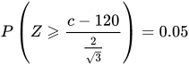
According to change-of-units rule for the normal distribution. Referring to Z-table, we can get
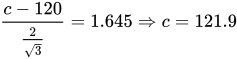
Here, the critical region. That is to say, if the recorded speed of a vehicle is greater than critical value 121.9, the driver will be fined. However, there are still 5% of the drivers are falsely fined since the recorded average speed is greater than 121.9 but the true speed does not pass 120, which we say, a type I error.
The type II error corresponds to the case that the true speed of a vehicle is over 120 kilometers per hour but the driver is not fined. For example, if the true speed of a vehicle μ=125, the probability that the driver is not fined can be calculated as

which means, if the true speed of a vehicle is 125, the driver has the probability of 0.36% to avoid the fine when the statistic is performed at level 125 since the recorded average speed is lower than 121.9. If the true speed is closer to 121.9 than 125, then the probability of avoiding the fine will also be higher.
The tradeoffs between type I error and type II error should also be considered. That is, in this case, if the traffic police do not want to falsely fine innocent drivers, the level α can be set to a smaller value, like 0.01. However, if that is the case, more drivers whose true speed is over 120 kilometers per hour, like 125, would be more likely to avoid the fine.
Etymology[edit]
In 1928, Jerzy Neyman (1894–1981) and Egon Pearson (1895–1980), both eminent statisticians, discussed the problems associated with «deciding whether or not a particular sample may be judged as likely to have been randomly drawn from a certain population»:[12] and, as Florence Nightingale David remarked, «it is necessary to remember the adjective ‘random’ [in the term ‘random sample’] should apply to the method of drawing the sample and not to the sample itself».[13]
They identified «two sources of error», namely:
- (a) the error of rejecting a hypothesis that should have not been rejected, and
- (b) the error of failing to reject a hypothesis that should have been rejected.
In 1930, they elaborated on these two sources of error, remarking that:
…in testing hypotheses two considerations must be kept in view, we must be able to reduce the chance of rejecting a true hypothesis to as low a value as desired; the test must be so devised that it will reject the hypothesis tested when it is likely to be false.
In 1933, they observed that these «problems are rarely presented in such a form that we can discriminate with certainty between the true and false hypothesis» . They also noted that, in deciding whether to fail to reject, or reject a particular hypothesis amongst a «set of alternative hypotheses», H1, H2…, it was easy to make an error:
…[and] these errors will be of two kinds:
- (I) we reject H0 [i.e., the hypothesis to be tested] when it is true,[14]
- (II) we fail to reject H0 when some alternative hypothesis HA or H1 is true. (There are various notations for the alternative).
In all of the papers co-written by Neyman and Pearson the expression H0 always signifies «the hypothesis to be tested».
In the same paper they call these two sources of error, errors of type I and errors of type II respectively.[15]
[edit]
Null hypothesis[edit]
It is standard practice for statisticians to conduct tests in order to determine whether or not a «speculative hypothesis» concerning the observed phenomena of the world (or its inhabitants) can be supported. The results of such testing determine whether a particular set of results agrees reasonably (or does not agree) with the speculated hypothesis.
On the basis that it is always assumed, by statistical convention, that the speculated hypothesis is wrong, and the so-called «null hypothesis» that the observed phenomena simply occur by chance (and that, as a consequence, the speculated agent has no effect) – the test will determine whether this hypothesis is right or wrong. This is why the hypothesis under test is often called the null hypothesis (most likely, coined by Fisher (1935, p. 19)), because it is this hypothesis that is to be either nullified or not nullified by the test. When the null hypothesis is nullified, it is possible to conclude that data support the «alternative hypothesis» (which is the original speculated one).
The consistent application by statisticians of Neyman and Pearson’s convention of representing «the hypothesis to be tested» (or «the hypothesis to be nullified») with the expression H0 has led to circumstances where many understand the term «the null hypothesis» as meaning «the nil hypothesis» – a statement that the results in question have arisen through chance. This is not necessarily the case – the key restriction, as per Fisher (1966), is that «the null hypothesis must be exact, that is free from vagueness and ambiguity, because it must supply the basis of the ‘problem of distribution,’ of which the test of significance is the solution.»[16] As a consequence of this, in experimental science the null hypothesis is generally a statement that a particular treatment has no effect; in observational science, it is that there is no difference between the value of a particular measured variable, and that of an experimental prediction.[citation needed]
Statistical significance[edit]
If the probability of obtaining a result as extreme as the one obtained, supposing that the null hypothesis were true, is lower than a pre-specified cut-off probability (for example, 5%), then the result is said to be statistically significant and the null hypothesis is rejected.
British statistician Sir Ronald Aylmer Fisher (1890–1962) stressed that the «null hypothesis»:
… is never proved or established, but is possibly disproved, in the course of experimentation. Every experiment may be said to exist only in order to give the facts a chance of disproving the null hypothesis.
— Fisher, 1935, p.19
Application domains[edit]
Medicine[edit]
In the practice of medicine, the differences between the applications of screening and testing are considerable.
Medical screening[edit]
Screening involves relatively cheap tests that are given to large populations, none of whom manifest any clinical indication of disease (e.g., Pap smears).
Testing involves far more expensive, often invasive, procedures that are given only to those who manifest some clinical indication of disease, and are most often applied to confirm a suspected diagnosis.
For example, most states in the USA require newborns to be screened for phenylketonuria and hypothyroidism, among other congenital disorders.
Hypothesis: «The newborns have phenylketonuria and hypothyroidism»
Null Hypothesis (H0): «The newborns do not have phenylketonuria and hypothyroidism»,
Type I error (false positive): The true fact is that the newborns do not have phenylketonuria and hypothyroidism but we consider they have the disorders according to the data.
Type II error (false negative): The true fact is that the newborns have phenylketonuria and hypothyroidism but we consider they do not have the disorders according to the data.
Although they display a high rate of false positives, the screening tests are considered valuable because they greatly increase the likelihood of detecting these disorders at a far earlier stage.
The simple blood tests used to screen possible blood donors for HIV and hepatitis have a significant rate of false positives; however, physicians use much more expensive and far more precise tests to determine whether a person is actually infected with either of these viruses.
Perhaps the most widely discussed false positives in medical screening come from the breast cancer screening procedure mammography. The US rate of false positive mammograms is up to 15%, the highest in world. One consequence of the high false positive rate in the US is that, in any 10-year period, half of the American women screened receive a false positive mammogram. False positive mammograms are costly, with over $100 million spent annually in the U.S. on follow-up testing and treatment. They also cause women unneeded anxiety. As a result of the high false positive rate in the US, as many as 90–95% of women who get a positive mammogram do not have the condition. The lowest rate in the world is in the Netherlands, 1%. The lowest rates are generally in Northern Europe where mammography films are read twice and a high threshold for additional testing is set (the high threshold decreases the power of the test).
The ideal population screening test would be cheap, easy to administer, and produce zero false-negatives, if possible. Such tests usually produce more false-positives, which can subsequently be sorted out by more sophisticated (and expensive) testing.
Medical testing[edit]
False negatives and false positives are significant issues in medical testing.
Hypothesis: «The patients have the specific disease».
Null hypothesis (H0): «The patients do not have the specific disease».
Type I error (false positive): «The true fact is that the patients do not have a specific disease but the physicians judges the patients was ill according to the test reports».
False positives can also produce serious and counter-intuitive problems when the condition being searched for is rare, as in screening. If a test has a false positive rate of one in ten thousand, but only one in a million samples (or people) is a true positive, most of the positives detected by that test will be false. The probability that an observed positive result is a false positive may be calculated using Bayes’ theorem.
Type II error (false negative): «The true fact is that the disease is actually present but the test reports provide a falsely reassuring message to patients and physicians that the disease is absent».
False negatives produce serious and counter-intuitive problems, especially when the condition being searched for is common. If a test with a false negative rate of only 10% is used to test a population with a true occurrence rate of 70%, many of the negatives detected by the test will be false.
This sometimes leads to inappropriate or inadequate treatment of both the patient and their disease. A common example is relying on cardiac stress tests to detect coronary atherosclerosis, even though cardiac stress tests are known to only detect limitations of coronary artery blood flow due to advanced stenosis.
Biometrics[edit]
Biometric matching, such as for fingerprint recognition, facial recognition or iris recognition, is susceptible to type I and type II errors.
Hypothesis: «The input does not identify someone in the searched list of people»
Null hypothesis: «The input does identify someone in the searched list of people»
Type I error (false reject rate): «The true fact is that the person is someone in the searched list but the system concludes that the person is not according to the data».
Type II error (false match rate): «The true fact is that the person is not someone in the searched list but the system concludes that the person is someone whom we are looking for according to the data».
The probability of type I errors is called the «false reject rate» (FRR) or false non-match rate (FNMR), while the probability of type II errors is called the «false accept rate» (FAR) or false match rate (FMR).
If the system is designed to rarely match suspects then the probability of type II errors can be called the «false alarm rate». On the other hand, if the system is used for validation (and acceptance is the norm) then the FAR is a measure of system security, while the FRR measures user inconvenience level.
Security screening[edit]
False positives are routinely found every day in airport security screening, which are ultimately visual inspection systems. The installed security alarms are intended to prevent weapons being brought onto aircraft; yet they are often set to such high sensitivity that they alarm many times a day for minor items, such as keys, belt buckles, loose change, mobile phones, and tacks in shoes.
Here, the null hypothesis is that the item is not a weapon, while the alternative hypothesis is that the item is a weapon.
A type I error (false positive): «The true fact is that the item is not a weapon but the system still alarms».
Type II error (false negative) «The true fact is that the item is a weapon but the system keeps silent at this time».
The ratio of false positives (identifying an innocent traveler as a terrorist) to true positives (detecting a would-be terrorist) is, therefore, very high; and because almost every alarm is a false positive, the positive predictive value of these screening tests is very low.
The relative cost of false results determines the likelihood that test creators allow these events to occur. As the cost of a false negative in this scenario is extremely high (not detecting a bomb being brought onto a plane could result in hundreds of deaths) whilst the cost of a false positive is relatively low (a reasonably simple further inspection) the most appropriate test is one with a low statistical specificity but high statistical sensitivity (one that allows a high rate of false positives in return for minimal false negatives).
Computers[edit]
The notions of false positives and false negatives have a wide currency in the realm of computers and computer applications, including computer security, spam filtering, Malware, Optical character recognition and many others.
For example, in the case of spam filtering the hypothesis here is that the message is a spam.
Thus, null hypothesis: «The message is not a spam».
Type I error (false positive): «Spam filtering or spam blocking techniques wrongly classify a legitimate email message as spam and, as a result, interferes with its delivery».
While most anti-spam tactics can block or filter a high percentage of unwanted emails, doing so without creating significant false-positive results is a much more demanding task.
Type II error (false negative): «Spam email is not detected as spam, but is classified as non-spam». A low number of false negatives is an indicator of the efficiency of spam filtering.
See also[edit]
- Binary classification
- Detection theory
- Egon Pearson
- Ethics in mathematics
- False positive paradox
- False discovery rate
- Family-wise error rate
- Information retrieval performance measures
- Neyman–Pearson lemma
- Null hypothesis
- Probability of a hypothesis for Bayesian inference
- Precision and recall
- Prosecutor’s fallacy
- Prozone phenomenon
- Receiver operating characteristic
- Sensitivity and specificity
- Statisticians’ and engineers’ cross-reference of statistical terms
- Testing hypotheses suggested by the data
- Type III error
References[edit]
- ^ «Type I Error and Type II Error». explorable.com. Retrieved 14 December 2019.
- ^ Chow, Y. W.; Pietranico, R.; Mukerji, A. (27 October 1975). «Studies of oxygen binding energy to hemoglobin molecule». Biochemical and Biophysical Research Communications. 66 (4): 1424–1431. doi:10.1016/0006-291x(75)90518-5. ISSN 0006-291X. PMID 6.
- ^ A modern introduction to probability and statistics : understanding why and how. Dekking, Michel, 1946-. London: Springer. 2005. ISBN 978-1-85233-896-1. OCLC 262680588.
{{cite book}}: CS1 maint: others (link) - ^ A modern introduction to probability and statistics : understanding why and how. Dekking, Michel, 1946-. London: Springer. 2005. ISBN 978-1-85233-896-1. OCLC 262680588.
{{cite book}}: CS1 maint: others (link) - ^ Sheskin, David (2004). Handbook of Parametric and Nonparametric Statistical Procedures. CRC Press. p. 54. ISBN 1584884401.
- ^ Smith, R. J.; Bryant, R. G. (27 October 1975). «Metal substitutions incarbonic anhydrase: a halide ion probe study». Biochemical and Biophysical Research Communications. 66 (4): 1281–1286. doi:10.1016/0006-291x(75)90498-2. ISSN 0006-291X. PMC 9650581. PMID 3.
- ^ Lindenmayer, David. (2005). Practical conservation biology. Burgman, Mark A. Collingwood, Vic.: CSIRO Pub. ISBN 0-643-09310-9. OCLC 65216357.
- ^ Chow, Y. W.; Pietranico, R.; Mukerji, A. (27 October 1975). «Studies of oxygen binding energy to hemoglobin molecule». Biochemical and Biophysical Research Communications. 66 (4): 1424–1431. doi:10.1016/0006-291x(75)90518-5. ISSN 0006-291X. PMID 6.
- ^ Smith, R. J.; Bryant, R. G. (27 October 1975). «Metal substitutions incarbonic anhydrase: a halide ion probe study». Biochemical and Biophysical Research Communications. 66 (4): 1281–1286. doi:10.1016/0006-291x(75)90498-2. ISSN 0006-291X. PMC 9650581. PMID 3.
- ^ Smith, R. J.; Bryant, R. G. (27 October 1975). «Metal substitutions incarbonic anhydrase: a halide ion probe study». Biochemical and Biophysical Research Communications. 66 (4): 1281–1286. doi:10.1016/0006-291x(75)90498-2. ISSN 0006-291X. PMC 9650581. PMID 3.
- ^ Moroi, K.; Sato, T. (15 August 1975). «Comparison between procaine and isocarboxazid metabolism in vitro by a liver microsomal amidase-esterase». Biochemical Pharmacology. 24 (16): 1517–1521. doi:10.1016/0006-2952(75)90029-5. ISSN 1873-2968. PMID 8.
- ^ NEYMAN, J.; PEARSON, E. S. (1928). «On the Use and Interpretation of Certain Test Criteria for Purposes of Statistical Inference Part I». Biometrika. 20A (1–2): 175–240. doi:10.1093/biomet/20a.1-2.175. ISSN 0006-3444.
- ^ C.I.K.F. (July 1951). «Probability Theory for Statistical Methods. By F. N. David. [Pp. ix + 230. Cambridge University Press. 1949. Price 155.]». Journal of the Staple Inn Actuarial Society. 10 (3): 243–244. doi:10.1017/s0020269x00004564. ISSN 0020-269X.
- ^ Note that the subscript in the expression H0 is a zero (indicating null), and is not an «O» (indicating original).
- ^ Neyman, J.; Pearson, E. S. (30 October 1933). «The testing of statistical hypotheses in relation to probabilities a priori». Mathematical Proceedings of the Cambridge Philosophical Society. 29 (4): 492–510. Bibcode:1933PCPS…29..492N. doi:10.1017/s030500410001152x. ISSN 0305-0041. S2CID 119855116.
- ^ Fisher, R.A. (1966). The design of experiments. 8th edition. Hafner:Edinburgh.
Bibliography[edit]
- Betz, M.A. & Gabriel, K.R., «Type IV Errors and Analysis of Simple Effects», Journal of Educational Statistics, Vol.3, No.2, (Summer 1978), pp. 121–144.
- David, F.N., «A Power Function for Tests of Randomness in a Sequence of Alternatives», Biometrika, Vol.34, Nos.3/4, (December 1947), pp. 335–339.
- Fisher, R.A., The Design of Experiments, Oliver & Boyd (Edinburgh), 1935.
- Gambrill, W., «False Positives on Newborns’ Disease Tests Worry Parents», Health Day, (5 June 2006). [1] Archived 17 May 2018 at the Wayback Machine
- Kaiser, H.F., «Directional Statistical Decisions», Psychological Review, Vol.67, No.3, (May 1960), pp. 160–167.
- Kimball, A.W., «Errors of the Third Kind in Statistical Consulting», Journal of the American Statistical Association, Vol.52, No.278, (June 1957), pp. 133–142.
- Lubin, A., «The Interpretation of Significant Interaction», Educational and Psychological Measurement, Vol.21, No.4, (Winter 1961), pp. 807–817.
- Marascuilo, L.A. & Levin, J.R., «Appropriate Post Hoc Comparisons for Interaction and nested Hypotheses in Analysis of Variance Designs: The Elimination of Type-IV Errors», American Educational Research Journal, Vol.7., No.3, (May 1970), pp. 397–421.
- Mitroff, I.I. & Featheringham, T.R., «On Systemic Problem Solving and the Error of the Third Kind», Behavioral Science, Vol.19, No.6, (November 1974), pp. 383–393.
- Mosteller, F., «A k-Sample Slippage Test for an Extreme Population», The Annals of Mathematical Statistics, Vol.19, No.1, (March 1948), pp. 58–65.
- Moulton, R.T., «Network Security», Datamation, Vol.29, No.7, (July 1983), pp. 121–127.
- Raiffa, H., Decision Analysis: Introductory Lectures on Choices Under Uncertainty, Addison–Wesley, (Reading), 1968.
External links[edit]
- Bias and Confounding – presentation by Nigel Paneth, Graduate School of Public Health, University of Pittsburgh
This article is about erroneous outcomes of statistical tests. For closely related concepts in binary classification and testing generally, see false positives and false negatives.
In statistical hypothesis testing, a type I error is the mistaken rejection of an actually true null hypothesis (also known as a «false positive» finding or conclusion; example: «an innocent person is convicted»), while a type II error is the failure to reject a null hypothesis that is actually false (also known as a «false negative» finding or conclusion; example: «a guilty person is not convicted»).[1] Much of statistical theory revolves around the minimization of one or both of these errors, though the complete elimination of either is a statistical impossibility if the outcome is not determined by a known, observable causal process.
By selecting a low threshold (cut-off) value and modifying the alpha (α) level, the quality of the hypothesis test can be increased.[2] The knowledge of type I errors and type II errors is widely used in medical science, biometrics and computer science.[clarification needed]
Intuitively, type I errors can be thought of as errors of commission, i.e. the researcher unluckily concludes that something is the fact. For instance, consider a study where researchers compare a drug with a placebo. If the patients who are given the drug get better than the patients given the placebo by chance, it may appear that the drug is effective, but in fact the conclusion is incorrect.
In reverse, type II errors are errors of omission. In the example above, if the patients who got the drug did not get better at a higher rate than the ones who got the placebo, but this was a random fluke, that would be a type II error. The consequence of a type II error depends on the size and direction of the missed determination and the circumstances. An expensive cure for one in a million patients may be inconsequential even if it truly is a cure.
Definition[edit]
Statistical background[edit]
In statistical test theory, the notion of a statistical error is an integral part of hypothesis testing. The test goes about choosing about two competing propositions called null hypothesis, denoted by H0 and alternative hypothesis, denoted by H1. This is conceptually similar to the judgement in a court trial. The null hypothesis corresponds to the position of the defendant: just as he is presumed to be innocent until proven guilty, so is the null hypothesis presumed to be true until the data provide convincing evidence against it. The alternative hypothesis corresponds to the position against the defendant. Specifically, the null hypothesis also involves the absence of a difference or the absence of an association. Thus, the null hypothesis can never be that there is a difference or an association.
If the result of the test corresponds with reality, then a correct decision has been made. However, if the result of the test does not correspond with reality, then an error has occurred. There are two situations in which the decision is wrong. The null hypothesis may be true, whereas we reject H0. On the other hand, the alternative hypothesis H1 may be true, whereas we do not reject H0. Two types of error are distinguished: type I error and type II error.[3]
Type I error[edit]
The first kind of error is the mistaken rejection of a null hypothesis as the result of a test procedure. This kind of error is called a type I error (false positive) and is sometimes called an error of the first kind. In terms of the courtroom example, a type I error corresponds to convicting an innocent defendant.
Type II error[edit]
The second kind of error is the mistaken failure to reject the null hypothesis as the result of a test procedure. This sort of error is called a type II error (false negative) and is also referred to as an error of the second kind. In terms of the courtroom example, a type II error corresponds to acquitting a criminal.[4]
Crossover error rate[edit]
The crossover error rate (CER) is the point at which type I errors and type II errors are equal. A system with a lower CER value provides more accuracy than a system with a higher CER value.
False positive and false negative[edit]
In terms of false positives and false negatives, a positive result corresponds to rejecting the null hypothesis, while a negative result corresponds to failing to reject the null hypothesis; «false» means the conclusion drawn is incorrect. Thus, a type I error is equivalent to a false positive, and a type II error is equivalent to a false negative.
Table of error types[edit]
Tabularised relations between truth/falseness of the null hypothesis and outcomes of the test:[5]
| Table of error types | Null hypothesis (H0) is |
||
|---|---|---|---|
| True | False | ||
| Decision about null hypothesis (H0) |
Don’t reject |
Correct inference (true negative) (probability = 1−α) |
Type II error (false negative) (probability = β) |
| Reject | Type I error (false positive) (probability = α) |
Correct inference (true positive) (probability = 1−β) |
Error rate[edit]
The results obtained from negative sample (left curve) overlap with the results obtained from positive samples (right curve). By moving the result cutoff value (vertical bar), the rate of false positives (FP) can be decreased, at the cost of raising the number of false negatives (FN), or vice versa (TP = True Positives, TPR = True Positive Rate, FPR = False Positive Rate, TN = True Negatives).
A perfect test would have zero false positives and zero false negatives. However, statistical methods are probabilistic, and it cannot be known for certain whether statistical conclusions are correct. Whenever there is uncertainty, there is the possibility of making an error. Considering this nature of statistics science, all statistical hypothesis tests have a probability of making type I and type II errors.[6]
- The type I error rate is the probability of rejecting the null hypothesis given that it is true. The test is designed to keep the type I error rate below a prespecified bound called the significance level, usually denoted by the Greek letter α (alpha) and is also called the alpha level. Usually, the significance level is set to 0.05 (5%), implying that it is acceptable to have a 5% probability of incorrectly rejecting the true null hypothesis.[7]
- The rate of the type II error is denoted by the Greek letter β (beta) and related to the power of a test, which equals 1−β.[8]
These two types of error rates are traded off against each other: for any given sample set, the effort to reduce one type of error generally results in increasing the other type of error.[9]
The quality of hypothesis test[edit]
The same idea can be expressed in terms of the rate of correct results and therefore used to minimize error rates and improve the quality of hypothesis test. To reduce the probability of committing a type I error, making the alpha value more stringent is quite simple and efficient. To decrease the probability of committing a type II error, which is closely associated with analyses’ power, either increasing the test’s sample size or relaxing the alpha level could increase the analyses’ power.[10] A test statistic is robust if the type I error rate is controlled.
Varying different threshold (cut-off) value could also be used to make the test either more specific or more sensitive, which in turn elevates the test quality. For example, imagine a medical test, in which an experimenter might measure the concentration of a certain protein in the blood sample. The experimenter could adjust the threshold (black vertical line in the figure) and people would be diagnosed as having diseases if any number is detected above this certain threshold. According to the image, changing the threshold would result in changes in false positives and false negatives, corresponding to movement on the curve.[11]
Example[edit]
Since in a real experiment it is impossible to avoid all type I and type II errors, it is important to consider the amount of risk one is willing to take to falsely reject H0 or accept H0. The solution to this question would be to report the p-value or significance level α of the statistic. For example, if the p-value of a test statistic result is estimated at 0.0596, then there is a probability of 5.96% that we falsely reject H0. Or, if we say, the statistic is performed at level α, like 0.05, then we allow to falsely reject H0 at 5%. A significance level α of 0.05 is relatively common, but there is no general rule that fits all scenarios.
Vehicle speed measuring[edit]
The speed limit of a freeway in the United States is 120 kilometers per hour. A device is set to measure the speed of passing vehicles. Suppose that the device will conduct three measurements of the speed of a passing vehicle, recording as a random sample X1, X2, X3. The traffic police will or will not fine the drivers depending on the average speed
In addition, we suppose that the measurements X1, X2, X3 are modeled as normal distribution N(μ,4). Then, T should follow N(μ,4/3) and the parameter μ represents the true speed of passing vehicle. In this experiment, the null hypothesis H0 and the alternative hypothesis H1 should be
H0: μ=120 against H1: μ1>120.
If we perform the statistic level at α=0.05, then a critical value c should be calculated to solve
According to change-of-units rule for the normal distribution. Referring to Z-table, we can get
Here, the critical region. That is to say, if the recorded speed of a vehicle is greater than critical value 121.9, the driver will be fined. However, there are still 5% of the drivers are falsely fined since the recorded average speed is greater than 121.9 but the true speed does not pass 120, which we say, a type I error.
The type II error corresponds to the case that the true speed of a vehicle is over 120 kilometers per hour but the driver is not fined. For example, if the true speed of a vehicle μ=125, the probability that the driver is not fined can be calculated as
which means, if the true speed of a vehicle is 125, the driver has the probability of 0.36% to avoid the fine when the statistic is performed at level 125 since the recorded average speed is lower than 121.9. If the true speed is closer to 121.9 than 125, then the probability of avoiding the fine will also be higher.
The tradeoffs between type I error and type II error should also be considered. That is, in this case, if the traffic police do not want to falsely fine innocent drivers, the level α can be set to a smaller value, like 0.01. However, if that is the case, more drivers whose true speed is over 120 kilometers per hour, like 125, would be more likely to avoid the fine.
Etymology[edit]
In 1928, Jerzy Neyman (1894–1981) and Egon Pearson (1895–1980), both eminent statisticians, discussed the problems associated with «deciding whether or not a particular sample may be judged as likely to have been randomly drawn from a certain population»:[12] and, as Florence Nightingale David remarked, «it is necessary to remember the adjective ‘random’ [in the term ‘random sample’] should apply to the method of drawing the sample and not to the sample itself».[13]
They identified «two sources of error», namely:
- (a) the error of rejecting a hypothesis that should have not been rejected, and
- (b) the error of failing to reject a hypothesis that should have been rejected.
In 1930, they elaborated on these two sources of error, remarking that:
…in testing hypotheses two considerations must be kept in view, we must be able to reduce the chance of rejecting a true hypothesis to as low a value as desired; the test must be so devised that it will reject the hypothesis tested when it is likely to be false.
In 1933, they observed that these «problems are rarely presented in such a form that we can discriminate with certainty between the true and false hypothesis» . They also noted that, in deciding whether to fail to reject, or reject a particular hypothesis amongst a «set of alternative hypotheses», H1, H2…, it was easy to make an error:
…[and] these errors will be of two kinds:
- (I) we reject H0 [i.e., the hypothesis to be tested] when it is true,[14]
- (II) we fail to reject H0 when some alternative hypothesis HA or H1 is true. (There are various notations for the alternative).
In all of the papers co-written by Neyman and Pearson the expression H0 always signifies «the hypothesis to be tested».
In the same paper they call these two sources of error, errors of type I and errors of type II respectively.[15]
[edit]
Null hypothesis[edit]
It is standard practice for statisticians to conduct tests in order to determine whether or not a «speculative hypothesis» concerning the observed phenomena of the world (or its inhabitants) can be supported. The results of such testing determine whether a particular set of results agrees reasonably (or does not agree) with the speculated hypothesis.
On the basis that it is always assumed, by statistical convention, that the speculated hypothesis is wrong, and the so-called «null hypothesis» that the observed phenomena simply occur by chance (and that, as a consequence, the speculated agent has no effect) – the test will determine whether this hypothesis is right or wrong. This is why the hypothesis under test is often called the null hypothesis (most likely, coined by Fisher (1935, p. 19)), because it is this hypothesis that is to be either nullified or not nullified by the test. When the null hypothesis is nullified, it is possible to conclude that data support the «alternative hypothesis» (which is the original speculated one).
The consistent application by statisticians of Neyman and Pearson’s convention of representing «the hypothesis to be tested» (or «the hypothesis to be nullified») with the expression H0 has led to circumstances where many understand the term «the null hypothesis» as meaning «the nil hypothesis» – a statement that the results in question have arisen through chance. This is not necessarily the case – the key restriction, as per Fisher (1966), is that «the null hypothesis must be exact, that is free from vagueness and ambiguity, because it must supply the basis of the ‘problem of distribution,’ of which the test of significance is the solution.»[16] As a consequence of this, in experimental science the null hypothesis is generally a statement that a particular treatment has no effect; in observational science, it is that there is no difference between the value of a particular measured variable, and that of an experimental prediction.[citation needed]
Statistical significance[edit]
If the probability of obtaining a result as extreme as the one obtained, supposing that the null hypothesis were true, is lower than a pre-specified cut-off probability (for example, 5%), then the result is said to be statistically significant and the null hypothesis is rejected.
British statistician Sir Ronald Aylmer Fisher (1890–1962) stressed that the «null hypothesis»:
… is never proved or established, but is possibly disproved, in the course of experimentation. Every experiment may be said to exist only in order to give the facts a chance of disproving the null hypothesis.
— Fisher, 1935, p.19
Application domains[edit]
Medicine[edit]
In the practice of medicine, the differences between the applications of screening and testing are considerable.
Medical screening[edit]
Screening involves relatively cheap tests that are given to large populations, none of whom manifest any clinical indication of disease (e.g., Pap smears).
Testing involves far more expensive, often invasive, procedures that are given only to those who manifest some clinical indication of disease, and are most often applied to confirm a suspected diagnosis.
For example, most states in the USA require newborns to be screened for phenylketonuria and hypothyroidism, among other congenital disorders.
Hypothesis: «The newborns have phenylketonuria and hypothyroidism»
Null Hypothesis (H0): «The newborns do not have phenylketonuria and hypothyroidism»,
Type I error (false positive): The true fact is that the newborns do not have phenylketonuria and hypothyroidism but we consider they have the disorders according to the data.
Type II error (false negative): The true fact is that the newborns have phenylketonuria and hypothyroidism but we consider they do not have the disorders according to the data.
Although they display a high rate of false positives, the screening tests are considered valuable because they greatly increase the likelihood of detecting these disorders at a far earlier stage.
The simple blood tests used to screen possible blood donors for HIV and hepatitis have a significant rate of false positives; however, physicians use much more expensive and far more precise tests to determine whether a person is actually infected with either of these viruses.
Perhaps the most widely discussed false positives in medical screening come from the breast cancer screening procedure mammography. The US rate of false positive mammograms is up to 15%, the highest in world. One consequence of the high false positive rate in the US is that, in any 10-year period, half of the American women screened receive a false positive mammogram. False positive mammograms are costly, with over $100 million spent annually in the U.S. on follow-up testing and treatment. They also cause women unneeded anxiety. As a result of the high false positive rate in the US, as many as 90–95% of women who get a positive mammogram do not have the condition. The lowest rate in the world is in the Netherlands, 1%. The lowest rates are generally in Northern Europe where mammography films are read twice and a high threshold for additional testing is set (the high threshold decreases the power of the test).
The ideal population screening test would be cheap, easy to administer, and produce zero false-negatives, if possible. Such tests usually produce more false-positives, which can subsequently be sorted out by more sophisticated (and expensive) testing.
Medical testing[edit]
False negatives and false positives are significant issues in medical testing.
Hypothesis: «The patients have the specific disease».
Null hypothesis (H0): «The patients do not have the specific disease».
Type I error (false positive): «The true fact is that the patients do not have a specific disease but the physicians judges the patients was ill according to the test reports».
False positives can also produce serious and counter-intuitive problems when the condition being searched for is rare, as in screening. If a test has a false positive rate of one in ten thousand, but only one in a million samples (or people) is a true positive, most of the positives detected by that test will be false. The probability that an observed positive result is a false positive may be calculated using Bayes’ theorem.
Type II error (false negative): «The true fact is that the disease is actually present but the test reports provide a falsely reassuring message to patients and physicians that the disease is absent».
False negatives produce serious and counter-intuitive problems, especially when the condition being searched for is common. If a test with a false negative rate of only 10% is used to test a population with a true occurrence rate of 70%, many of the negatives detected by the test will be false.
This sometimes leads to inappropriate or inadequate treatment of both the patient and their disease. A common example is relying on cardiac stress tests to detect coronary atherosclerosis, even though cardiac stress tests are known to only detect limitations of coronary artery blood flow due to advanced stenosis.
Biometrics[edit]
Biometric matching, such as for fingerprint recognition, facial recognition or iris recognition, is susceptible to type I and type II errors.
Hypothesis: «The input does not identify someone in the searched list of people»
Null hypothesis: «The input does identify someone in the searched list of people»
Type I error (false reject rate): «The true fact is that the person is someone in the searched list but the system concludes that the person is not according to the data».
Type II error (false match rate): «The true fact is that the person is not someone in the searched list but the system concludes that the person is someone whom we are looking for according to the data».
The probability of type I errors is called the «false reject rate» (FRR) or false non-match rate (FNMR), while the probability of type II errors is called the «false accept rate» (FAR) or false match rate (FMR).
If the system is designed to rarely match suspects then the probability of type II errors can be called the «false alarm rate». On the other hand, if the system is used for validation (and acceptance is the norm) then the FAR is a measure of system security, while the FRR measures user inconvenience level.
Security screening[edit]
False positives are routinely found every day in airport security screening, which are ultimately visual inspection systems. The installed security alarms are intended to prevent weapons being brought onto aircraft; yet they are often set to such high sensitivity that they alarm many times a day for minor items, such as keys, belt buckles, loose change, mobile phones, and tacks in shoes.
Here, the null hypothesis is that the item is not a weapon, while the alternative hypothesis is that the item is a weapon.
A type I error (false positive): «The true fact is that the item is not a weapon but the system still alarms».
Type II error (false negative) «The true fact is that the item is a weapon but the system keeps silent at this time».
The ratio of false positives (identifying an innocent traveler as a terrorist) to true positives (detecting a would-be terrorist) is, therefore, very high; and because almost every alarm is a false positive, the positive predictive value of these screening tests is very low.
The relative cost of false results determines the likelihood that test creators allow these events to occur. As the cost of a false negative in this scenario is extremely high (not detecting a bomb being brought onto a plane could result in hundreds of deaths) whilst the cost of a false positive is relatively low (a reasonably simple further inspection) the most appropriate test is one with a low statistical specificity but high statistical sensitivity (one that allows a high rate of false positives in return for minimal false negatives).
Computers[edit]
The notions of false positives and false negatives have a wide currency in the realm of computers and computer applications, including computer security, spam filtering, Malware, Optical character recognition and many others.
For example, in the case of spam filtering the hypothesis here is that the message is a spam.
Thus, null hypothesis: «The message is not a spam».
Type I error (false positive): «Spam filtering or spam blocking techniques wrongly classify a legitimate email message as spam and, as a result, interferes with its delivery».
While most anti-spam tactics can block or filter a high percentage of unwanted emails, doing so without creating significant false-positive results is a much more demanding task.
Type II error (false negative): «Spam email is not detected as spam, but is classified as non-spam». A low number of false negatives is an indicator of the efficiency of spam filtering.
See also[edit]
- Binary classification
- Detection theory
- Egon Pearson
- Ethics in mathematics
- False positive paradox
- False discovery rate
- Family-wise error rate
- Information retrieval performance measures
- Neyman–Pearson lemma
- Null hypothesis
- Probability of a hypothesis for Bayesian inference
- Precision and recall
- Prosecutor’s fallacy
- Prozone phenomenon
- Receiver operating characteristic
- Sensitivity and specificity
- Statisticians’ and engineers’ cross-reference of statistical terms
- Testing hypotheses suggested by the data
- Type III error
References[edit]
- ^ «Type I Error and Type II Error». explorable.com. Retrieved 14 December 2019.
- ^ Chow, Y. W.; Pietranico, R.; Mukerji, A. (27 October 1975). «Studies of oxygen binding energy to hemoglobin molecule». Biochemical and Biophysical Research Communications. 66 (4): 1424–1431. doi:10.1016/0006-291x(75)90518-5. ISSN 0006-291X. PMID 6.
- ^ A modern introduction to probability and statistics : understanding why and how. Dekking, Michel, 1946-. London: Springer. 2005. ISBN 978-1-85233-896-1. OCLC 262680588.
{{cite book}}: CS1 maint: others (link) - ^ A modern introduction to probability and statistics : understanding why and how. Dekking, Michel, 1946-. London: Springer. 2005. ISBN 978-1-85233-896-1. OCLC 262680588.
{{cite book}}: CS1 maint: others (link) - ^ Sheskin, David (2004). Handbook of Parametric and Nonparametric Statistical Procedures. CRC Press. p. 54. ISBN 1584884401.
- ^ Smith, R. J.; Bryant, R. G. (27 October 1975). «Metal substitutions incarbonic anhydrase: a halide ion probe study». Biochemical and Biophysical Research Communications. 66 (4): 1281–1286. doi:10.1016/0006-291x(75)90498-2. ISSN 0006-291X. PMC 9650581. PMID 3.
- ^ Lindenmayer, David. (2005). Practical conservation biology. Burgman, Mark A. Collingwood, Vic.: CSIRO Pub. ISBN 0-643-09310-9. OCLC 65216357.
- ^ Chow, Y. W.; Pietranico, R.; Mukerji, A. (27 October 1975). «Studies of oxygen binding energy to hemoglobin molecule». Biochemical and Biophysical Research Communications. 66 (4): 1424–1431. doi:10.1016/0006-291x(75)90518-5. ISSN 0006-291X. PMID 6.
- ^ Smith, R. J.; Bryant, R. G. (27 October 1975). «Metal substitutions incarbonic anhydrase: a halide ion probe study». Biochemical and Biophysical Research Communications. 66 (4): 1281–1286. doi:10.1016/0006-291x(75)90498-2. ISSN 0006-291X. PMC 9650581. PMID 3.
- ^ Smith, R. J.; Bryant, R. G. (27 October 1975). «Metal substitutions incarbonic anhydrase: a halide ion probe study». Biochemical and Biophysical Research Communications. 66 (4): 1281–1286. doi:10.1016/0006-291x(75)90498-2. ISSN 0006-291X. PMC 9650581. PMID 3.
- ^ Moroi, K.; Sato, T. (15 August 1975). «Comparison between procaine and isocarboxazid metabolism in vitro by a liver microsomal amidase-esterase». Biochemical Pharmacology. 24 (16): 1517–1521. doi:10.1016/0006-2952(75)90029-5. ISSN 1873-2968. PMID 8.
- ^ NEYMAN, J.; PEARSON, E. S. (1928). «On the Use and Interpretation of Certain Test Criteria for Purposes of Statistical Inference Part I». Biometrika. 20A (1–2): 175–240. doi:10.1093/biomet/20a.1-2.175. ISSN 0006-3444.
- ^ C.I.K.F. (July 1951). «Probability Theory for Statistical Methods. By F. N. David. [Pp. ix + 230. Cambridge University Press. 1949. Price 155.]». Journal of the Staple Inn Actuarial Society. 10 (3): 243–244. doi:10.1017/s0020269x00004564. ISSN 0020-269X.
- ^ Note that the subscript in the expression H0 is a zero (indicating null), and is not an «O» (indicating original).
- ^ Neyman, J.; Pearson, E. S. (30 October 1933). «The testing of statistical hypotheses in relation to probabilities a priori». Mathematical Proceedings of the Cambridge Philosophical Society. 29 (4): 492–510. Bibcode:1933PCPS…29..492N. doi:10.1017/s030500410001152x. ISSN 0305-0041. S2CID 119855116.
- ^ Fisher, R.A. (1966). The design of experiments. 8th edition. Hafner:Edinburgh.
Bibliography[edit]
- Betz, M.A. & Gabriel, K.R., «Type IV Errors and Analysis of Simple Effects», Journal of Educational Statistics, Vol.3, No.2, (Summer 1978), pp. 121–144.
- David, F.N., «A Power Function for Tests of Randomness in a Sequence of Alternatives», Biometrika, Vol.34, Nos.3/4, (December 1947), pp. 335–339.
- Fisher, R.A., The Design of Experiments, Oliver & Boyd (Edinburgh), 1935.
- Gambrill, W., «False Positives on Newborns’ Disease Tests Worry Parents», Health Day, (5 June 2006). [1] Archived 17 May 2018 at the Wayback Machine
- Kaiser, H.F., «Directional Statistical Decisions», Psychological Review, Vol.67, No.3, (May 1960), pp. 160–167.
- Kimball, A.W., «Errors of the Third Kind in Statistical Consulting», Journal of the American Statistical Association, Vol.52, No.278, (June 1957), pp. 133–142.
- Lubin, A., «The Interpretation of Significant Interaction», Educational and Psychological Measurement, Vol.21, No.4, (Winter 1961), pp. 807–817.
- Marascuilo, L.A. & Levin, J.R., «Appropriate Post Hoc Comparisons for Interaction and nested Hypotheses in Analysis of Variance Designs: The Elimination of Type-IV Errors», American Educational Research Journal, Vol.7., No.3, (May 1970), pp. 397–421.
- Mitroff, I.I. & Featheringham, T.R., «On Systemic Problem Solving and the Error of the Third Kind», Behavioral Science, Vol.19, No.6, (November 1974), pp. 383–393.
- Mosteller, F., «A k-Sample Slippage Test for an Extreme Population», The Annals of Mathematical Statistics, Vol.19, No.1, (March 1948), pp. 58–65.
- Moulton, R.T., «Network Security», Datamation, Vol.29, No.7, (July 1983), pp. 121–127.
- Raiffa, H., Decision Analysis: Introductory Lectures on Choices Under Uncertainty, Addison–Wesley, (Reading), 1968.
External links[edit]
- Bias and Confounding – presentation by Nigel Paneth, Graduate School of Public Health, University of Pittsburgh
Статистика — сложная наука об измерении и анализе различных данных. Как и во многих других дисциплинах, в этой отрасли существует понятие гипотезы. Так, гипотеза в статистике — это какое-либо положение, которое нужно принять или отвергнуть. Причём в данной отрасли есть несколько видов таких допущений, схожих между собой по определению, но отличающихся на практике. Нулевая гипотеза — сегодняшний предмет изучения.
От общего к частному: гипотезы в статистике
От основного определения предположений отходит ещё одно, не менее важное, — статистическая гипотеза есть изучение генеральной совокупности важных для науки объектов, относительно коих учёными делаются выводы. Ее можно проверить с помощью выборки (части генеральной совокупности). Приведём несколько примеров статистических гипотез:
 1. Успеваемость всего класса, возможно, зависит от уровня образования каждого учащегося.
2. Начальный курс математики в равной степени усваивается как детьми, пришедшими в школу в 6 лет, так и детьми, пришедшими в 7.
Простой гипотезой в статистике называют такое предположение, которое однозначно характеризует определённый параметр величины, взятой учёным.
Сложная состоит из нескольких или бесконечного множества простых. Указывается некоторая область или нет точного ответа.
Полезно понимать несколько определений гипотез в статистике, чтобы не путать их на практике.
Концепция нулевой гипотезы
Нулевая гипотеза — это теория о том, что есть некие две совокупности, которые не различаются между собой. Однако на научном уровне нет понятия «не различаются», но есть «их сходство равно нулю». От этого определения и было образовано понятие. В статистике нулевая гипотеза обозначается как Н0. Причём крайним значением невозможного (маловероятного) считается от 0.01 до 0.05 или менее.
Лучше разобрать, что такое нулевая гипотеза, пример из жизни поможет. Педагог в университете предположил, что различный уровень подготовки учащихся двух групп к зачётной работе вызван незначительными параметрами, случайными причинами, не влияющими на общий уровень образования (разница в подготовке двух групп студентов равна нулю).
Однако встречно стоит привести пример альтернативной гипотезы — допущения, опровергающего утверждение нулевой теории (Н1). Например: директор университета предположил, что различный уровень в подготовке к зачётной работе у учащихся двух групп вызван применением педагогами разных методик обучения (разница в подготовке двух групп существенна и на то есть объяснение).
 Теперь сразу видна разница между понятиями «нулевая гипотеза» и «альтернативная гипотеза». Примеры иллюстрируют эти понятия.
Проверка нулевой гипотезы
Создать предположение — это ещё полбеды. Настоящей проблемой для новичков считается проверка нулевой гипотезы. Именно тут многих и ожидают трудности.
Используя метод альтернативной гипотезы, утверждающей нечто обратное нулевой теории, можно сравнить оба варианта и выбрать верный. Так действует статистика.
Пусть нулевая гипотеза Н0, а альтернативная Н1, тогда:
Н0: c = c0;
Н1: c ≠ c0.
Здесь c — это некое среднее значение генеральной совокупности, которое предстоит найти, а c0 — данное изначально значение, по отношению к которому проверяется гипотеза. Также есть некоторое число Х — среднее значение выборки, по которому определяется c0.
Итак, проверка заключается в сравнении Х и c0, если Х=c0 ,то принимается нулевая гипотеза. Если же Х≠c0, то по условию верной считается альтернативная.
«Доверительный» способ проверки
Существует наиболее действенный способ, с помощью которого нулевая статистическая гипотеза легко проверяется на практике. Он заключается в построении диапазона значений до 95% точности.
Для начала понадобится знать формулу расчёта доверительного интервала:
X — t*Sx ≤ c ≤ X + t*Sx,
где Х — данное изначально число на основе альтернативной гипотезы;
t — табличные величины (коэффициент Стьюдента);
Sx — стандартная средняя ошибка, которая рассчитывается как Sx = σ/√n, где в числителе стандартное отклонение, а в знаменателе — объём выборки.
Итак, предположим ситуацию. До ремонта конвейер в день выпускал 32.1 кг конечной продукции, а после ремонта, как утверждает предприниматель, коэффициент полезного действия вырос, и конвейер, по недельной проверке, начал выпускать 39.6 кг в среднем.
 Нулевая гипотеза будет утверждать, что ремонт никак не повлиял на КПД конвейера. Альтернативная гипотеза скажет, что ремонт коренным образом изменил КПД конвейера, поэтому производительность его повысилась.
По таблице находим n=7, t = 2,447, откуда формула примет следующий вид:
39,6 – 2,447*4,2 ≤ с ≤ 39,6 + 2,447*4,2;
29,3 ≤ с ≤ 49,9.
Получается, что значение 32.1 входит в диапазон, а следовательно, значение, предложенное альтернативой — 39.6 — не принимается автоматически. Помните, что сначала проверяется на правильность нулевая гипотеза, а потом — противоположная.
Разновидности отрицания
До этого рассматривался такой вариант построения гипотезы, где Н0 утверждает что-либо, а Н1 это опровергает. Откуда можно было составить подобную систему:
Н0: с = с0;
Н1: с ≠ с0.
Но существует ещё два родственных способа опровержения. К примеру, нулевая гипотеза утверждает, что средняя оценка успеваемости класса больше 4.54, а альтернативная тогда скажет, что средняя успеваемость того же класса менее 4.54. И выглядеть в виде системы это будет так:
Н0: с ⩾ 4.54;
Н1: с < 4.54.
Обратите внимание, что нулевая гипотеза утверждает, что значение больше или равно, а статистическая — что строго меньше. Строгость знака неравенства имеет большое значение!
Статистическая проверка
Статистическая проверка нулевых гипотез заключается в использовании статистического критерия. Такие критерии подчиняются различным законам распределения.
 К примеру, существует F-критерий, который рассчитывается по распределению Фишера. Есть T-критерий, чаще всего используемый на практике, зависящий от распределения Стьюдента. Квадратный критерий согласия Пирсона и т. д.
Область принятия нулевой гипотезы
В алгебре есть понятие «область допустимых значений». Это такой отрезок или точка на оси Х, на котором находится множество значений статистики, при которых нулевая гипотеза верна. Крайние точки отрезка — критические значения. Лучи по правую и левую сторону отрезка — критические области. Если найденное значение входит в них, то нулевая теория опровергается и принимается альтернативная.
Опровержение нулевой гипотезы
Нулевая гипотеза в статистике временами очень изворотливое понятие. Во время проверки её можно допустить ошибки двух типов:
 1. Отвержение верной нулевой гипотезы. Обозначим первый тип как а=1.
2. Принятие ложной нулевой гипотезы. Второй тип обозначим как а=2.
Стоит понимать, что это не одинаковые параметры, исходы ошибок могут существенно различаться между собой и иметь разные выборки.
Пример ошибок двух типов
Со сложными понятиями легче разобраться на примере.
Во время производства некоего лекарства от учёных требуется чрезвычайная осторожность, так как превышение дозы одного из компонентов провоцирует высокий уровень токсичности готового препарата, от которого пациенты, принимающие его, могут умереть. Однако на химическом уровне выявить передозировку невозможно.
Из-за этого перед тем как выпустить лекарство в продажу, небольшую его дозу проверяют на крысах или кроликах, вводя им препарат. Если большая часть испытуемых умирает, то лекарство в продажу не допускается, если подопытные живы, то лекарство разрешают продавать в аптеках.
 Первый случай: на самом деле лекарство было не токсично, но во время эксперимента была допущена оплошность и препарат классифицировали как токсичный и не допустили в продажу. А=1.
Второй случай: в ходе другого эксперимента при проверке другой партии лекарства решено, что препарат не токсичен, и в продажу его допустили, хотя на самом деле препарат был ядовит. А=2.
Первый вариант повлечёт за собой крупные финансовые затраты поставщика-предпринимателя, так как придётся уничтожить всю партию лекарства и начинать с нуля.
Вторая ситуация спровоцирует смерть пациентов, купивших и употреблявших это лекарство.
Теория вероятности
Не только нулевые, но все гипотезы в статистике и экономике разделяют по уровню значимости.
Уровень значимости — процент появления ошибок первого рода (отклонение верной нулевой гипотезы).
• первый уровень — 5% или 0.05, т. е. вероятность ошибиться 5 к 100 или 1 к 20.
• второй уровень — 1% или 0.01, т. е. вероятность 1 к 100.
• третий уровень — 0.1% или 0.001, вероятность 1 к 1000.
Критерии проверки гипотезы
Если учёным уже был сделан вывод о правильности нулевой гипотезы, то её необходимо подвергнуть проверке. Это необходимо, чтобы исключить ошибку. Существует основной критерий проверки нулевой гипотезы, состоящий из нескольких этапов:
1. Берётся допустимая ошибочная вероятность P=0.05.
2. Подбирается статистика для критерия 1.
3. По известному методу находится область допустимых значений.
4. Теперь вычисляется значение статистики Т.
5. Если Т (статистика) принадлежит области принятия нулевой гипотезы (как в «доверительном» методе), то предположения считаются верными, а значит, и сама нулевая гипотеза остаётся верной.

Именно так действует статистика. Нулевая гипотеза при грамотной проверке будет принята или отвергнута.
Стоит заметить, что для обычных предпринимателей и пользователей первые три этапа бывает очень сложно выполнить безошибочно, поэтому их доверяют профессиональным математикам. Зато 4 и 5 этапы может выполнить любой человек, в достаточной мере знающий статистические методы проверки.